1

Paper 194-30

Comparing the SAS® Forecasting System with PROC HPF and SAS® Enterprise Miner

Patricia B. Cerrito, University of Louisville, Louisville, KY

ABSTRACT SAS has now developed multiple methods for investigating time series data. This includes the ETS forecasting system, the time series node in Enterprise Miner (version 5.1), and the recently developed HPF (high-performance forecasting). It is the purpose of this paper to compare and contrast the different methods while demonstrating their use. The aim of these methods is to create accurate forecasts that can be used in business and industry for budgeting purposes. In this paper, one time series example will be explored in detail using the various time series methods. Differences and similarities in methods will be examined. Forecasts will be compared and contrasted.

INTRODUCTION SAS has developed the time Series Forecasting System (SAS/ETS) to examine time series data. The system is defined to determine the optimal method for forecasting. More recently, SAS has developed the High Performance Forecasting system (HPF) that also chooses the optimal method for forecasting. It can also work with transactional data where the data points are not at equally spaced time intervals. The two methods will be compared and contrasted in this paper, In addition, the HPF procedure will be discussed in detail.

DEFINITION OF TIME SERIES MODELS. A time series model can take into consideration the following characteristics:

1. Autocorrelation. A positive deviation from the mean is likely to stay positive; a negative deviation is likely to stay negative.

2. Trend. A positive or negative trend requires a first or second difference. 3. Seasonality. The data have a seasonal trend. 4. Transformation. To maintain the assumption of normality, a transformation is sometimes

required. A model that is purely autoregressive (with autocorrelations) means that the current value Y(t) is dependent upon a specific number of previous values so that in the case of an autoregression of size p, Y(t)=µ+α1(Y(t-1)-µ)+α2(Y(t-2)-µ)+…+αp(Y(t-p)-µ)+ε(t). (1) The number of lags used in the model is estimated based upon the autocorrelations. The moving average component expresses the current value Y(t) in terms of future shocks (or errors): Y(t)=µ+ε(t)-θ1ε(t-1)-…-θqε(t-q). (2) In the existence of a trend, a first or second difference is used. That is, a new model W(t) is defined so that W(t)=Y(t)-Y(t-1) (3) and the model is then defined for the difference W(t). Once this is estimated, Y(t) is estimated as equal to Y(t)=W(t)+Y(t-1). The number of differences is defined by the parameter d. The three components (1), (2), and (3) make up the ARIMA model (AR=autoregressive, I=integrated, MA=moving average). It is identified as of order (p,d,q). It estimates both the autocorrelation and trend. Seasonality is added to the model by using an ARIMA(p,d,q)x(P,D,Q) model, where P=number of seasonal autoregressive terms, D=number of seasonal differences, Q=number of seasonal moving average terms. In the seasonal part of the model, all of these factors operate across multiples of lag s (the number of periods in a season). If the seasonality changes on a yearly basis, then the value of s is equal to 12. If the seasonal pattern is both strong and stable over time (e.g., high in the Summer and low in the Winter, or vice versa), then the model should probably use a seasonal difference regardless of whether the first, non-seasonal part uses a difference, since this will prevent the seasonal pattern from "dying out" in the long-term forecasts.

Statistics and Data AnalysisSUGI 30

2

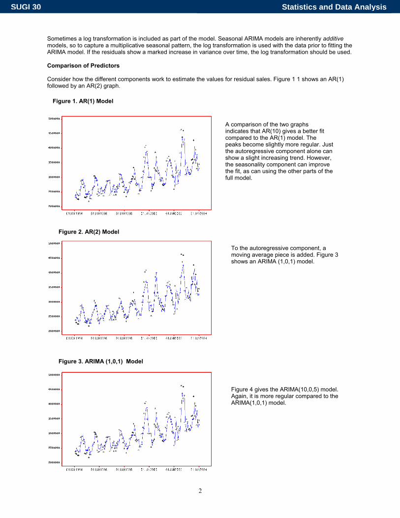
Sometimes a log transformation is included as part of the model. Seasonal ARIMA models are inherently additive models, so to capture a multiplicative seasonal pattern, the log transformation is used with the data prior to fitting the ARIMA model. If the residuals show a marked increase in variance over time, the log transformation should be used. Comparison of Predictors Consider how the different components work to estimate the values for residual sales. Figure 1 1 shows an AR(1) followed by an AR(2) graph.

A comparison of the two graphs indicates that AR(10) gives a better fit compared to the AR(1) model. The peaks become slightly more regular. Just the autoregressive component alone can show a slight increasing trend. However, the seasonality component can improve the fit, as can using the other parts of the full model.

Figure 4 gives the ARIMA(10,0,5) model. Again, it is more regular compared to the ARIMA(1,0,1) model.

Figure 1. AR(1) Model

Figure 2. AR(2) Model

To the autoregressive component, a moving average piece is added. Figure 3 shows an ARIMA (1,0,1) model.

Figure 3. ARIMA (1,0,1) Model

Statistics and Data AnalysisSUGI 30

3

The two models that use multiplicative seasonal adjustment deal with seasonality in an explicit fashion--i.e., seasonal indices are broken out as an explicit part of the model. The ARIMA models deal with seasonality in a more implicit manner--we can't easily see in the ARIMA output how the average December, say, differs from the average July. Depending on whether it is deemed important to isolate the seasonal pattern, this might be a factor in choosing among models. The ARIMA models have the advantage that, once they have been initialized, they have fewer "moving parts" than the exponential smoothing and adjustment models. The optimal method for this time series uses Winter’s method which adds a smoothing component to the trend and seasonality components. This model is shown

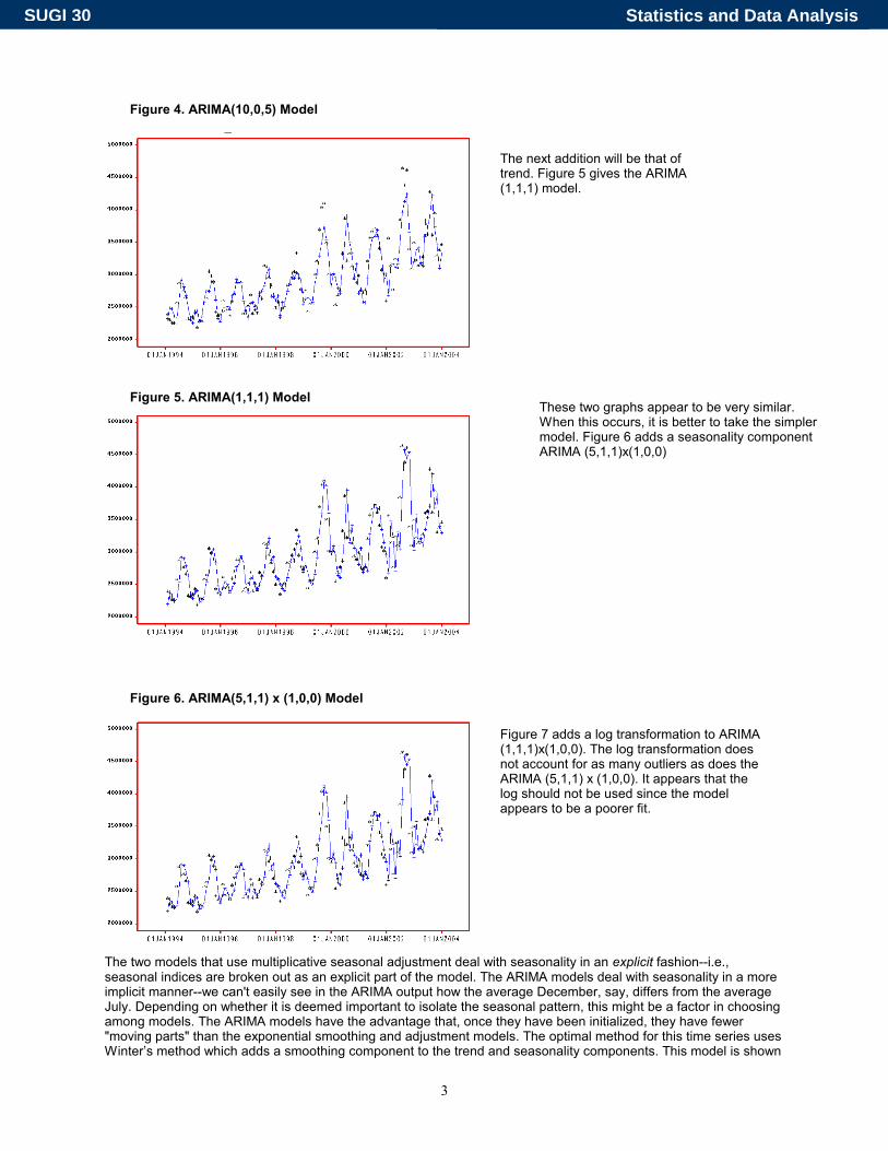
These two graphs appear to be very similar. When this occurs, it is better to take the simpler model. Figure 6 adds a seasonality component ARIMA (5,1,1)x(1,0,0)

Figure 4. ARIMA(10,0,5) Model

The next addition will be that of trend. Figure 5 gives the ARIMA (1,1,1) model.

Figure 5. ARIMA(1,1,1) Model

Figure 6. ARIMA(5,1,1) x (1,0,0) Model

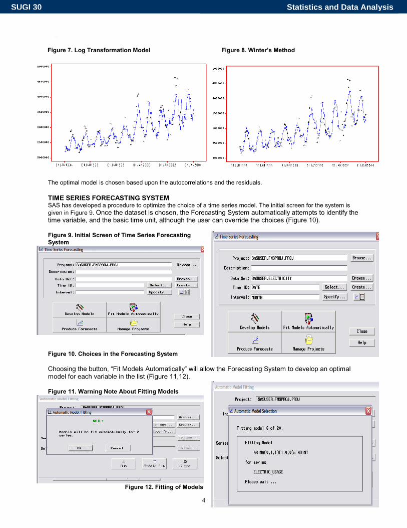
Figure 7 adds a log transformation to ARIMA (1,1,1)x(1,0,0). The log transformation does not account for as many outliers as does the ARIMA (5,1,1) x (1,0,0). It appears that the log should not be used since the model appears to be a poorer fit.

Statistics and Data AnalysisSUGI 30

4

in Figure 8.

The optimal model is chosen based upon the autocorrelations and the residuals.

TIME SERIES FORECASTING SYSTEM SAS has developed a procedure to optimize the choice of a time series model. The initial screen for the system is given in Figure 9. Once the dataset is chosen, the Forecasting System automatically attempts to identify the time variable, and the basic time unit, although the user can override the choices (Figure 10). Figure 9. Initial Screen of Time Series Forecasting System

Figure 10. Choices in the Forecasting System Choosing the button, “Fit Models Automatically” will allow the Forecasting System to develop an optimal model for each variable in the list (Figure 11,12). Figure 11. Warning Note About Fitting Models

Figure 12. Fitting of Models

Figure 7. Log Transformation Model

Figure 8. Winter’s Method

Statistics and Data AnalysisSUGI 30

5

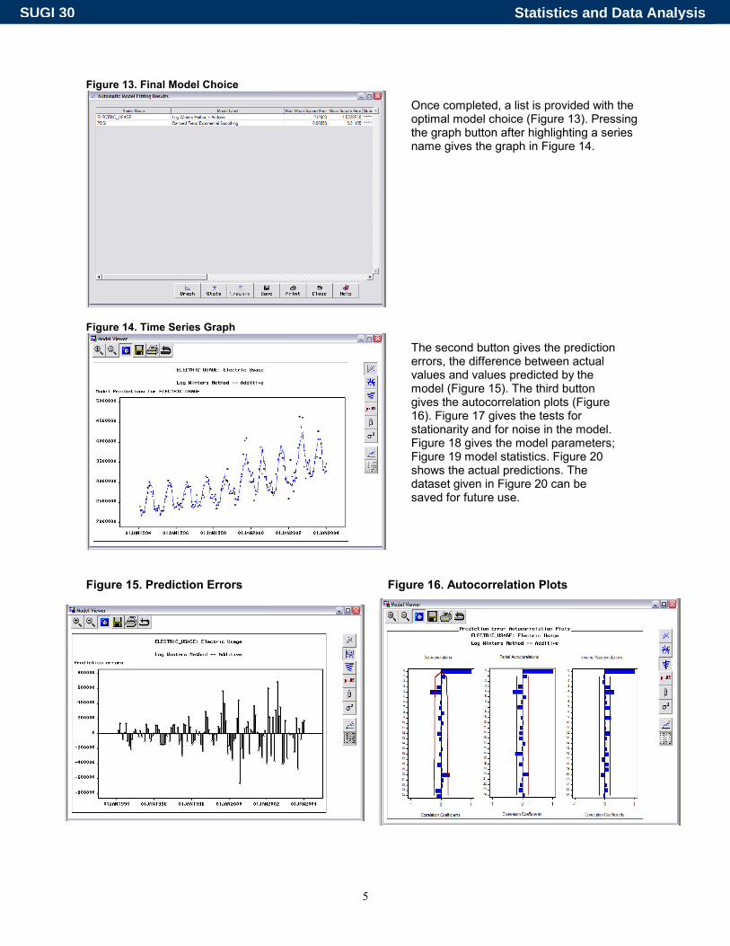
Figure 13. Final Model Choice

Figure 14. Time Series Graph

Figure 15. Prediction Errors Figure 16. Autocorrelation Plots

Once completed, a list is provided with the optimal model choice (Figure 13). Pressing the graph button after highlighting a series name gives the graph in Figure 14.

The second button gives the prediction errors, the difference between actual values and values predicted by the model (Figure 15). The third button gives the autocorrelation plots (Figure 16). Figure 17 gives the tests for stationarity and for noise in the model. Figure 18 gives the model parameters; Figure 19 model statistics. Figure 20 shows the actual predictions. The dataset given in Figure 20 can be saved for future use.

Statistics and Data AnalysisSUGI 30

6

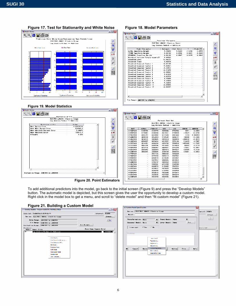
Figure 17. Test for Stationarity and White Noise Figure 18. Model Parameters

Figure 19. Model Statistics

Figure 20. Point Estimators To add additional predictors into the model, go back to the initial screen (Figure 9) and press the “Develop Models” button. The automatic model is depicted, but this screen gives the user the opportunity to develop a custom model. Right click in the model box to get a menu, and scroll to “delete model” and then “fit custom model” (Figure 21). Figure 21. Building a Custom Model

Statistics and Data AnalysisSUGI 30

7

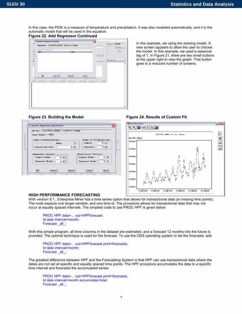
In this case, the PDSI is a measure of temperature and precipitation. It was also modeled automatically, and it is the automatic model that will be used in the equation. Figure 22. Add Regressor Continued

Figure 23. Building the Model Figure 24. Results of Custom Fit

HIGH PERFORMANCE FORECASTING With version 9.1., Enterprise Miner has a time series option that allows for transactional data (ie missing time points). The node expects one target variable, and one time id. The procedure allows for transactional data that may not occur at equally spaced intervals. The simplest code to use PROC HPF is given below:

PROC HPF data=... out=HPFforecast; Id date interval=month; Forecast _all_;

With this simple program, all time columns in the dataset are estimated, and a forecast 12 months into the future is provided. The optimal technique is used for the forecast. To use the ODS operating system to list the forecasts, add

PROC HPF data=... out=HPFforecast print=forecasts; Id date interval=month; Forecast _all_;

The greatest difference between HPF and the Forecasting System is that HPF can use transactional data where the dates are not set at specific and equally spaced time points. The HPF procedure accumulates the data to a specific time interval and forecasts the accumulated series:

PROC HPF data=... out=HPFforecast print=forecasts; Id date interval=month accumulate=total; Forecast _all_;

In this example, we using the existing model. A new screen appears to allow the user to choose the model. In this example, we used a seasonal lag of 1. In Figure 21, there are two small buttons at the upper right to view the graph. That button goes to a reduced number of screens.

Statistics and Data AnalysisSUGI 30

8

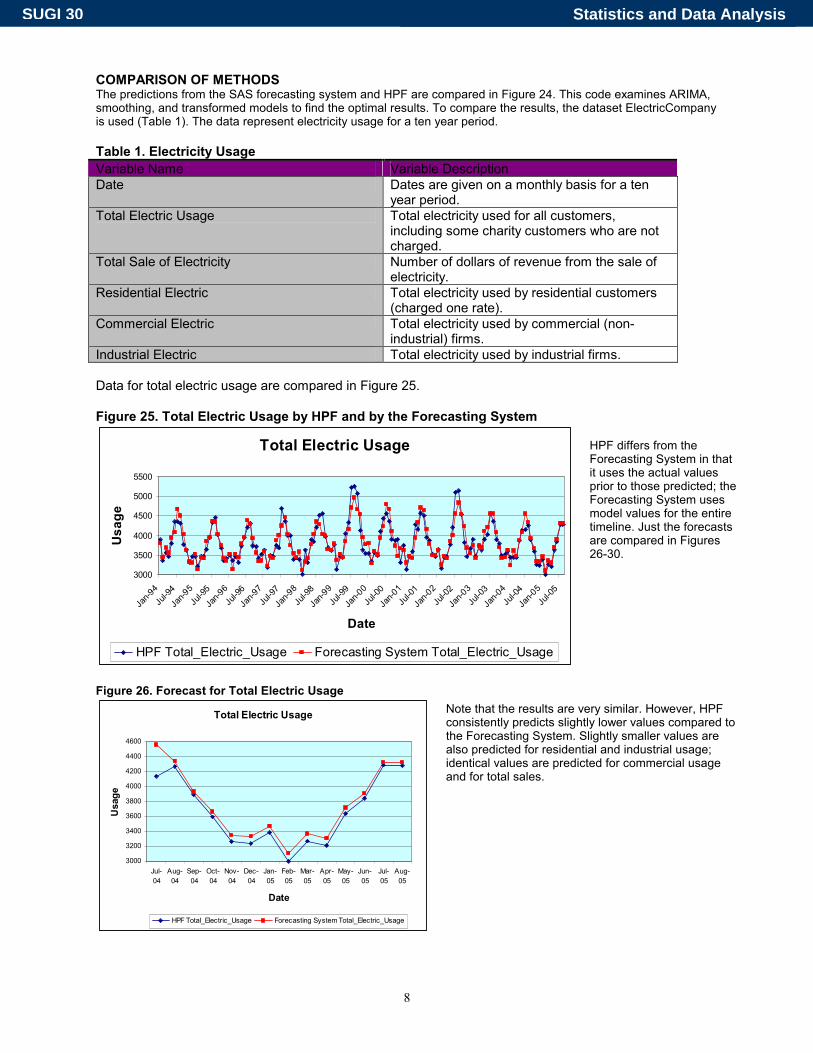
COMPARISON OF METHODS The predictions from the SAS forecasting system and HPF are compared in Figure 24. This code examines ARIMA, smoothing, and transformed models to find the optimal results. To compare the results, the dataset ElectricCompany is used (Table 1). The data represent electricity usage for a ten year period. Table 1. Electricity Usage Variable Name Variable Description Date Dates are given on a monthly basis for a ten

year period. Total Electric Usage Total electricity used for all customers,

including some charity customers who are not charged.

Total Sale of Electricity Number of dollars of revenue from the sale of electricity.

Residential Electric Total electricity used by residential customers (charged one rate).

Commercial Electric Total electricity used by commercial (non-industrial) firms.

Industrial Electric Total electricity used by industrial firms. Data for total electric usage are compared in Figure 25. Figure 25. Total Electric Usage by HPF and by the Forecasting System

Total Electric Usage

3000

3500

4000

4500

5000

5500

Jan-9

4Ju

l-94

Jan-9

5Ju

l-95

Jan-9

6Ju

l-96

Jan-9

7Ju

l-97

Jan-9

8Ju

l-98

Jan-9

9Ju

l-99

Jan-0

0Ju

l-00

Jan-0

1Ju

l-01

Jan-0

2Ju

l-02

Jan-0

3Ju

l-03

Jan-0

4Ju

l-04

Jan-0

5Ju

l-05

Date

Usa

ge

HPF Total_Electric_Usage Forecasting System Total_Electric_Usage

Figure 26. Forecast for Total Electric Usage

Total Electric Usage

3000

3200

3400

3600

3800

4000

4200

4400

4600

Jul-04

Aug-04

Sep-04

Oct-04

Nov-04

Dec-04

Jan-05

Feb-05

Mar-05

Apr-05

May-05

Jun-05

Jul-05

Aug-05

Date

Usa

ge

HPF Total_Electric_Usage Forecasting System Total_Electric_Usage

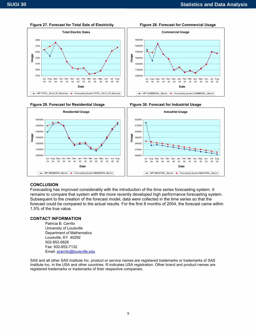
HPF differs from the Forecasting System in that it uses the actual values prior to those predicted; the Forecasting System uses model values for the entire timeline. Just the forecasts are compared in Figures 26-30.

Note that the results are very similar. However, HPF consistently predicts slightly lower values compared to the Forecasting System. Slightly smaller values are also predicted for residential and industrial usage; identical values are predicted for commercial usage and for total sales.

Statistics and Data AnalysisSUGI 30

9

Figure 27. Forecast for Total Sale of Electricity Figure 28. Forecast for Commercial Usage

Total Electric Sales

2700

2900

3100

3300

3500

3700

3900

Jul-04

Aug-04

Sep-04

Oct-04

Nov-04

Dec-04

Jan-05

Feb-05

Mar-05

Apr-05

May-05

Jun-05

Jul-05

Aug-05

Date

Usa

ge

HPF TOTAL_SALE_OF_Electricity Forecasting System TOTAL_SALE_OF_Electricity

Commercial Usage

1000000

1100000

1200000

1300000

1400000

1500000

1600000

Jul-04

Aug-04

Sep-04

Oct-04

Nov-04

Dec-04

Jan-05

Feb-05

Mar-05

Apr-05

May-05

Jun-05

Jul-05

Aug-05

Date

Usa

ge

HPF COMMERCIAL_Electric Forecasting System COMMERCIAL_Electric

Figure 29. Forecast for Residential Usage Figure 30. Forecast for Industrial Usage

Residential Usage

1000000

1100000

1200000

1300000

1400000

1500000

1600000

Jul-04

Aug-04

Sep-04

Oct-04

Nov-04

Dec-04

Jan-05

Feb-05

Mar-05

Apr-05

May-05

Jun-05

Jul-05

Aug-05

Date

Usa

ge

HPF RESIDENTIAl_Electric Forecasting System RESIDENTIAl_Electric

Industrial Usage

360000

370000

380000

390000

400000

410000

420000

Jul-04

Aug-04

Sep-04

Oct-04

Nov-04

Dec-04

Jan-05

Feb-05

Mar-05

Apr-05

May-05

Jun-05

Jul-05

Aug-05

Date

Usa

ge

HPF INDUSTRIAL_Electric Forecasting System INDUSTRIAL_Electric

CONCLUSION Forecasting has improved considerably with the introduction of the time series forecasting system. It remains to compare that system with the more recently developed high performance forecasting system. Subsequent to the creation of the forecast model, data were collected in the time series so that the forecast could be compared to the actual results. For the first 8 months of 2004, the forecast came within 1.5% of the true value.

CONTACT INFORMATION Patricia B. Cerrito University of Louisville Department of Mathematics Louisville, KY 40292 502-852-6826 Fax: 502-852-7132 Email: pcerrito@louisville.edu

SAS and all other SAS Institute Inc. product or service names are registered trademarks or trademarks of SAS Institute Inc. in the USA and other countries. ® indicates USA registration. Other brand and product names are registered trademarks or trademarks of their respective companies.

Statistics and Data AnalysisSUGI 30