1584 IEEE TRANSACTIONS ON AUDIO, SPEECH, AND LANGUAGE ... · 1584 IEEE TRANSACTIONS ON AUDIO, SPEECH, AND LANGUAGE PROCESSING, VOL. 19, NO. 6, AUGUST 2011 Transient Noise Reduction

1584 IEEE TRANSACTIONS ON AUDIO, SPEECH, AND LANGUAGE PROCESSING, VOL. 19, NO. 6, AUGUST 2011

Transient Noise Reduction UsingNonlocal Diffusion Filters

Ronen Talmon, Student Member, IEEE, Israel Cohen, Senior Member, IEEE, andSharon Gannot, Senior Member, IEEE

Abstract—Enhancement of speech signals for hands-free com-munication systems has attracted significant research efforts in thelast few decades. Still, many aspects and applications remain openand require further research. One of the important open problemsis the single-channel transient noise reduction. In this paper, wepresent a novel approach for transient noise reduction that relies onnon-local (NL) neighborhood filters. In particular, we propose analgorithm for the enhancement of a speech signal contaminated byrepeating transient noise events. We assume that the time durationof each reoccurring transient event is relatively short compared tospeech phonemes and model the speech source as an auto-regres-sive (AR) process. The proposed algorithm consists of two stages.In the first stage, we estimate the power spectral density (PSD) ofthe transient noise by employing a NL neighborhood filter. In thesecond stage, we utilize the optimally modified log spectral am-plitude (OM-LSA) estimator for denoising the speech using thenoise PSD estimate from the first stage. Based on a statistical modelfor the measurements and diffusion interpretation of NL filtering,we obtain further insight into the algorithm behavior. In partic-ular, for given transient noise, we determine whether estimationof the noise PSD is feasible using our approach, how to properlyset the algorithm parameters, and what is the expected perfor-mance of the algorithm. Experimental study shows good resultsin enhancing speech signals contaminated by transient noise, suchas typical household noises, construction sounds, keyboard typing,and metronome clacks.

Index Terms—Acoustic noise, impulse noise, speech enhance-ment, speech processing, transient noise.

I. INTRODUCTION

E NHANCEMENT of speech signals is of great interest inmany hands-free communication systems. Although this

problem has attracted significant research efforts for severaldecades, many aspects remain open and require further research.Among them is the single-channel transient noise reduction.Traditional speech enhancement approaches usually consist oftwo components: noise power spectrum estimation and estima-tion of the desired clean speech signal. In single-channel-basedapplications, spectral information is usually exploited for theestimation of the noise [1]–[6]. In particular, the noise signal is

Manuscript received February 23, 2010; revised October 30, 2010; acceptedNovember 02, 2010. Date of publication November 18, 2010; date of currentversion June 01, 2011. The associate editor coordinating the review of this man-uscript and approving it for publication was Dr. Michael Seltzer.

R. Talmon and I. Cohen are with the Department of Electrical Engineering,Technion-Israel Institute of Technology, Haifa 32000, Israel (e-mail: [email protected]; [email protected]).

S. Gannot is with the School of Engineering, Bar-Ilan University, Ramat-Gan,52900, Israel (e-mail: [email protected]).

Color versions of one or more of the figures in this paper are available onlineat http://ieeexplore.ieee.org.

Digital Object Identifier 10.1109/TASL.2010.2093651

assumed to remain stationary during the observation interval;hence, its power spectral density (PSD) is time-invariant orslowly varying compared to the speech. Another common andfundamental assumption is that the speech signal is not presentduring the whole observation interval. A common approach forestimating the noise PSD is to average the noisy measurementover periods where the speech is absent. Using the noise PSDestimate, the speech signal can be estimated based on somestatistical model.

The assumption of stationary noise signal poses a major lim-itation on these traditional algorithms, making them inadequatein many transient noise environments. Transient noises areusually characterized by percussive or impulsive nature, i.e., asudden burst of sound. Typically, transients consist of an initialpeak followed by decaying short-duration oscillations of lengthranging from 10 to 50 ms. Among them we mention noise orig-inating from engines, keyboard typing, construction operations,bells, knocking, rings, hammering, etc. Vaseghi and Rayner [7],[8] proposed a method for detection and suppression of suchimpulsive noise, consisting of relatively short duration noisepulses. After detecting a transient, the corrupted segment iscompletely removed and the source signal is estimated using in-terpolation that relies on the assumption that the desired sourceis auto-regressive (AR). Godsill and Rayner [9] improved thealgorithm based on a statistical model and interpolation usinga Gibbs sampler. Unfortunately, removing the entire corruptedsegment is problematic since acceptable speech completion isobtained only for very short transient occurrences.

Traditional methods typically do not take into account therepetitive nature of many transient noises. Usually a distinct pat-tern appears a large number of times at different time locations.The fact that the same pattern appears multiple times can be uti-lized for improved denoising. Specifically, the pattern intervalscan be identified, and the transient noise may be extracted byaveraging over all of these instances.

This approach naturally leads to nonlocal (NL) denoisingmethods using an NL neighborhood filter [10]. This methodcombined with local kernels, enables signal denoising withspecially tailored locality metrics adapted to specific tasks athand [11]–[14]. These methods are also known as bilateralfiltering. The main idea in nonlocal filtering is to process thedata according to the affinity metric conveyed by a kernel,which enables to capture similar patterns. This results incombining together data samples from different locations intime. Hence, this process is referred to as “nonlocal,” whereas“local” filtering is associated with processing of data sam-ples from adjacent locations. Although NL averaging is verysimple, it is surprisingly superior to other methods. A diffusion

1558-7916/$26.00 © 2010 IEEE

TALMON et al.: TRANSIENT NOISE REDUCTION USING NONLOCAL DIFFUSION FILTERS 1585

interpretation of the NL denoising approaches [15], explainsthe behavior of NL neighborhood filters and enables improvedfiltering algorithms. The analysis of Singer et al. [15] is mainlybased on a probabilistic model and on the relation betweenthe averaging process and the eigenstructure of the denoisingfilter. Although NL neighborhood filters have recently becomecommon in image processing applications, their potential inaudio processing in general, and speech enhancement in partic-ular, has not yet been fully investigated.

In this paper, we present a novel approach for speech en-hancement that relies on NL filters. In particular we propose analgorithm for the enhancement of nonstationary AR source con-taminated with repeating transient noise events. For simplicity,we assume that the time duration of each reoccurring transientevent is relatively short compared to speech phonemes and thatall events have the same spectral features up to random ampli-fications, as presented by Vaseghi and Rayner [8]. It is worth-while noting that we evaluate the proposed algorithm using realsignal recordings, since these restrictive assumptions may seeminadequate in practical scenarios. The proposed algorithm con-sists of two stages. In the first stage, we estimate the PSD ofthe transient noise. This is achieved by enhancing the transientnoise, relying on the strong auto-correlation of the speech signalin time and the burst-like nature of the transient noise. Then,we employ an NL neighborhood filter to extract the transientnoise signal. Unlike the approach proposed in [8], we aim at es-timating the transient signal rather than just detecting the loca-tions in time of transient events. The NL filter, employed with aspecially tailored similarity function, enables to implicitly cap-ture the underlying structure of the measurements. This struc-ture conveys significant information, which may help to distin-guish between the transient noise and the speech source signal.In the second stage, we utilize the optimally modified log spec-tral amplitude (OM-LSA) estimator [4] for denoising the speechwith a modified noise PSD estimator, that relies on the extractedtransient signal. We note that the noise estimate from the firststage can also be incorporated into other algorithms. For ex-ample, in [16], a transient noise reduction algorithm was pro-posed relying on a given indicator for transient noise events. Ourapproach may provide an indicator for transient noise eventsbased on NL filtering.

The proposed algorithm is robust to various transient noisetypes. We show good results in cleaning a speech signal con-taminated with transient noise, such as keyboard typing, typicalhousehold noises, construction sounds, and metronome clacks.In addition, we present a probabilistic analysis of the NL fil-tering by introducing a statistical model for the measurements.Based on the diffusion interpretation indicated by Singer et al.[15], we obtain further insight into the algorithm behavior. Inparticular, for given transient noise, we determine whether es-timation of the noise PSD is feasible using our approach, howto properly set the algorithm parameters, and what is the ex-pected performance of the algorithm. Recently, we have pre-sented a transient noise reduction algorithm that relies on a mod-ified NL filter [17]. The modified filter is incorporated to obtainfurther enhancement and robustness. This work extends [17] andprovides a probabilistic analysis.

This paper is organized as follows. In Section II, we describethe geometric approach for data analysis in general, and a dif-fusion framework in particular. In Section III, we formulate theproblem of transient noise reduction. In Section IV, we presentthe proposed algorithm and analyze it in Section V based on dif-fusion interpretation of the NL filters. Finally, in Section VI ex-perimental results are presented, demonstrating the performanceof the proposed algorithm.

II. DIFFUSION FRAMEWORK

In recent years, there has been a growing effort to developdata analysis methods based on the geometry of the acquiredraw data. These geometric approaches or manifold learningmethods aim at discovering the underlying structure in datasets as a precursor to other types of processing [18]–[24]. Inparticular, among the geometric approaches, diffusion maps[24], [25] is of particular interest, since its derivation and someof its main results pave the way for diffusion interpretation ofthe NL filtering [15]. The proposed algorithm does not involvethe actual mapping of diffusion maps; however, it relies on thederivation and main results of this method. Thus, in this section,we present the general formulation of the diffusion framework.

Let be a given high-dimensional data set ofsamples, where and is a field. We note that in thegeneral setting, is merely an index of a sample in the data set.The diffusion framework consists of the following steps: 1) con-struction of a weighted graph on the given data set , based ona pairwise weight function , that corresponds to a local affinitybetween samples in ; 2) derivation of a random-walk on thegraph via a construction of a transition matrix that is derivedfrom ; and 3) interpretation of the discrete random-walk on thegraph as a continuous diffusion process on a manifold.

A. Building a Graph

We construct the graph on the data set in order to cap-ture the geometry of the set. Let be akernel or a weight function representing a notion of pairwiseaffinity between the data samples, with a scale parameter . Forall , the weight function has the following prop-erties: 1) symmetry: ; 2) non-nega-tivity: ; 3) fast decay: given a positive scaleparameter , for and

for . For example, a Gaussiankernel satisfies theseproperties. It is worthwhile noting that the Euclidean distancecan be replaced by any application-oriented metric. For sim-plicity, we omit the notation of the scale , when referring tothe kernel .

Based on the relation defined by the kernel, we form aweighted graph or a Euclidean manifold, where the data sam-ples are the graph vertices and the kernel sets the weightsof the edges connecting the data points, i.e., the weight of theedge connecting the node to the node is . It isworthwhile noting that the kernel conveys the local geometry ofthe data set , unlike global methods such as principalcomponent analysis (PCA), which are based on statistical


correlations between data samples. Moreover, a kernel withfast decay [property (3)] intensifies the locality property ofthis approach, as it defines a neighborhood around each datasample of radius (in other words, samples subject to

are weakly connected to ). Thus, the choiceof the specific kernel function should be application-oriented toyield meaningful connections and represent perceptual affinity.

B. Constructing a Random Walk

Following classical construction in spectral graph theory[26], the kernel is normalized to create a non-symmetric pair-wise metric, given by

(1)

where is often referred to as the degreeof . Using the non-negativity property of the kernel, whichyields that , and since , thefunction can be interpreted as a transition probability func-tion of a Markov chain1 on the data set . Specifi-cally, the states of the Markov chain are the graph nodesand represents the probability of transition in a singlerandom-walk step from node to node . We point out that

is not described in a conventional conditional probability no-tation to emphasize its role as a non-symmetric pairwise metricand to correspond with the common notations from the litera-ture. Let denote the matrix corresponding to the kernel func-tion , where its element is , and let

be the matrix corresponding to the function , bothon the finite data set , where is a diagonal matrixwith . Let be a matrix con-sisting of the data set samples

(2)

Advancing the random-walk on the data set a single step forwardcan be written as . Similarly, propagating the random-walk

steps forward corresponds to raising to the power of andapplying it on the data set as . We denote the probabilityfunction corresponding to as , which measures theprobability of transition from node to node in steps.

Let denote the Markovian process defined by the transi-tion matrix , with time index . The probabilistic interpreta-tion of a single step is:2

(3)

which means that running the chain forward gives the expectedvalues of the random-walker starting at the node after a single

1A Markov chain is a discrete random process subject to the next state dependsonly on the current state.

2�� extracts the �� row of the matrix�.

step. Consequently, performing steps corresponds to the ex-pected value after steps. Hopefully, this process results in re-vealing the relevant geometric structure of . As weshow in Section IV, (3) may be interpreted as a single iteration ofan NL filter. In Appendix I, we present a simple example of de-noising a telegraph signal corrupted by additive white Gaussiannoise to demonstrate the diffusion framework construction.

C. Diffusion Interpretation

Results from spectral theory can be employed to describe ,enabling to study the geometric structure of in a com-pact and efficient way. It can be shown that has a completesequence of left and right eigenvectors and positiveeigenvalues, written in a descending order

(4)

satisfying and . The eigenvaluesand the eigenvectors provide a spectral repre-

sentation of the geometry of the manifold defined by the dataset and the kernel function .

Let be the probability density function of the data setsamples. When using an exponentially decaying kernel, e.g., aGaussian kernel, it is shown in [24], [25] that for a large dataset (corresponds to dense sampling of the manifold)and small-scale (corresponds to very local kernel), thetransition matrix of the discrete random-walk on the graphconverges to the continuous backward Fokker–Planck operator

, defined for any smooth function by

(5)

where is defined as , is the gradientof , and is the inner product. Let bethe potential derived from the probability density functionof the data set samples on the manifold. Then Fokker–Planckoperator (5) can be written as

(6)

For example, the Fokker–Planck operator may describe themotion of a particle in a potential field, where the functiondenotes the location of the particle. An analysis of the diffusionprocess associated with the Fokker–Planck operator, and thecharacteristics of its eigenfunctions have been extensivelystudied in the literature [27]. The characteristics of the spectraldecomposition of the diffusion operator may be exploitedfor various tasks and applications [15], [25], [28]–[30]. InSection V, we exploit this convergence for the analysis oftransient noise extraction using an NL filter.

III. PROBLEM FORMULATION

Throughout this paper, we use the following notation con-vention. Lowercase letters denote scalars, bold letters vectors,and capital bold letters matrices. In addition, signals in the timedomain are represented by lowercase letters followed by thetime index in brackets, whereas signals in the short-time Fouriertransform (STFT) domain are represented by lower-case letters


(to emphasize time variation) followed by a subscript indicatingthe time frame and frequency bin indices.

Let denote a speech signal and let be a contami-nating interference, represented by

(7)

where is a dominating transient part, and is a lowvariance stationary noise. The signal measured by a microphoneis given by

(8)

For simplicity, in the remainder of this paper we omit the sta-tionary part. The proposed algorithm is designed for distinctionof the transient noise from the rest of the measurement compo-nents. Evidently, it is much easier to distinguish the stationarynoise from the transients, compared to the nonstationary speech.Consequently, the presence of stationary noise does not changesignificantly the derivation of the algorithm. In Section VI, weshow that the proposed algorithm can handle speech contami-nated by both transient and stationary noises. It is worthwhilenoting that in the literature numerous methods for enhancementof speech signals contaminated by (quasi) stationary noise canbe found. In addition, we can employ one of these methods priorto the proposed algorithm.

We assume that the speech signal is modeled as an AR processin short-time frames [31]. The observation interval is dividedinto short-time frames of length . Accordingly, in eachtime frame , the source signal is an AR process,given by

(9)

where is a white noise excitation signal with zero-meanand variance, and are AR coefficients in frame

. We assume is large enough to capture the long-term linearprediction coefficients, enabling representation of both voicedand unvoiced phonemes. In practice, we verify that the numberof coefficients is greater than a single period of the pitch to en-able its representation. In addition, we do not exploit the white-ness of the excitation signal, but rather rely on the fact that theexcitation signal can be distinct from the transient noise.

The transient noise consists of short duration pulses ofrandom amplitudes. It may be modeled as the output of a filterexcited by an amplitude-modulated random binary sequence[7], [8], [32], given by

(10)

where is a binary valued random sequence oftime locations of the transient noise events, is a continuousvalued random process of transient amplitudes, and is animpulse response of a filter that models the duration and shapeof each transient event. In this paper, we use a fixed impulseresponse , which implies that the transient events havethe same spectral features up to random amplitude. Hence, thetransient noise can be viewed as a superposition of the im-pulse response with random amplitudes. This restrictive

assumption is used for simplicity. It is worthwhile noting thatin Section VI the proposed algorithm is evaluated in practicalscenarios using real transient noise recordings. We use theGaussian–Poisson statistical model proposed in [8], i.e., therandom amplitude is modeled as a Gaussian process with

mean and variance, and the transient time locationsare modeled as a Poisson process.3 The Poisson distributionis assumed for simplicity; however, it does not have a signif-icant role in the algorithm derivations, nor does the Gaussianamplitude and the exact pulse shape. For sufficiently low-ratePoisson process, we assume that no more than one transientevent exists in each short time frames. We denote by theset of time frames free of transient noise occurrences, and by

, we denote the set of time frames that include transientoccurrences.

IV. PROPOSED ALGORITHM

The proposed algorithm consists of two stages. In the firststage, we aim at estimating the PSD of the transient noise. Inthe second stage, we utilize the OM-LSA estimator [4] for de-noising the speech. The OM-LSA that we use is equipped witha modified noise PSD estimator, based on the estimation of thetransient noise PSD obtained in the first stage.

A. Transient Noise Spectrum Estimation

Aiming at enhancing the characteristic difference betweenthe transient noise and the AR source signal, we “whiten” (or“decorrelate”) the noisy measurement in each time frameusing the AR parameters of the source signal. Let be thewhitened measurement in time frame , which can be writtenas4

(11)

Substituting (7)–(9) into (11) yields

(12)

where is a smeared version of the transient noise, givenby

(13)

In (12), we observe that the whitened signal consists of twocomponents—the source excitation signal , and a smearedversion of the transient noise .

The derivation of (11) and (12) is applicable given the AR co-efficients of the source signal , which are unknown. Esti-mation of the coefficients of an AR source from noisy measure-ments has been a subject of many studies and extends the scopeof this paper. In practice, we use the common Levinson–Durbinalgorithm to estimate the AR coefficients in time frames freeof a transient noise event. By exploiting the short duration oftransient impulses and by assuming slow variations of the AR

3We use a discrete time version of the continuous time Poisson process, asdescribed in [8].

4We note that in our notation, tilde denotes a whitened version of the signal.


coefficients in time, we are able to set the AR coefficients intime frames that contain a transient occurrence according to theestimated AR coefficients of neighboring frames.5 Moreover, aspreviously noted, the main role of the whitening is to further en-hance the distinction between transient noise events and speechcomponents. Therefore in practice, the proposed algorithm isnot sensitive to estimation errors of the AR coefficients.

According to our assumption, typical transient events haveunique spectral features. Thus, we apply the STFT to emphasizethe difference between the transient noise and the source. Weuse STFT time-frames of length . Let be the whitenedmeasurement in the STFT domain in time frame and frequencybin . Using (12) and (13), it can be written as

(14)

where is the STFT of the excitation signal, is the mul-tiplicative transfer function (MTF) approximation of the sourceAR filter [33], and is the STFT of the transient noise. Using(10), is given by

(15)

where is the MTF approximation of the transient noisesystem , is the random amplitude of theimpulse, and is the random relative location of the impulsefrom the beginning of the frame, both in frame . In (15)we assume a single impulse per frame. In addition, we circum-vent overlaps of the transient occurrences between frames byincluding in only frames that contain a significant part ofa transient event. Since time frames usually overlap, combinedwith the fact that typical transient events are shorter than thelength of a time frame, we are able to assume that frames inshare the characteristic spectral features of a transient event.

Given the AR coefficients of the source, estimating thePSD of the transient noise and estimating the PSD of thesmeared version of the transient noise are equivalenttasks. Furthermore, (12) and (14) imply that the whitenedmeasurements consist of the smeared version of the transientnoise “contaminated” by a white noise . Consequently,we can interpret the estimation of the transient noise PSD asa problem of spectral denoising, where we aim at enhancingthe transient events and attenuating the white excitation signal.For that purpose, we employ an NL filter that exploits thedivergence between the STFT features of the transient eventsand the white excitation signal.

Consider the STFT features of each time frame as a singlesample in a high-dimensional field. Specifically, let be avector of the STFT coefficients from all frequency bins in the

time-frame of the whitened signal , defined as

(16)

5We note that speech onset or phoneme transition right before or after thetransient results in inaccurate estimation of the AR coefficients. We assume suchcases occur with very low probability.

and let be an matrix consisting of all these vectors,given by

(17)

We define an affinity kernel between pairs of samplesand for all and . In this paper, we use the following

Gaussian kernel based on a Euclidean distance:

(18)

where is a vector of size , given by

(19)

where is the short-time PSD of in time-frameand the frequency bin . In practice, we evaluate the short-timePSD by smoothing the periodograms over timeframes according to the common Welch method. This spe-cific choice of kernel is motivated by the desire to exploit thereoccurring distinct spectral features of time frames containinga transient event, which may be appropriately conveyed by thepower spectrum . In addition, the phase of the framesthat contain transient events should be disregarded in the com-parison, since it varies from frame to frame, and depends on therelative location of each event in the frame. Consequently, thephase of the STFT has little role in the estimation of the tran-sient noise PSD derived in this step of the proposed algorithm.However, the phase is taken into consideration in the applica-tion of the NL filter, and in the next step, where the speech isestimated according to the OM-LSA gain function calculation.

As described in Section II, we view the STFT features ofthe time frames as nodes of an undirected symmetricgraph. Two nodes and are connected by an edge withweight , that corresponds to the affinity betweenand . We continue with the construction of a random-walkon the graph nodes by normalizing the kernel , similarlyto (1). We obtain a non-symmetric metric betweentwo nodes, which represents the probability of transition in asingle step from to . Let be the Markovian processassociated with this random-walk (where represents timeindex), and let be an matrix consisting of thetransition probabilities. Similarly to (3), a single random-walkstep is given by

(20)

In (20), a single step is interpreted as averaging over similar timeframe samples, where the sense of similarity is emerged fromthe kernel. Thus, the choice of the kernel is of key impor-tance in this method. We rely on the fact that time frames that


contain transient events consist of distinct spectral features com-pared to time frames free of transient events, as demonstratedin Section VI. Consequently, the kernel (18), which comparesbetween the spectral features of time frames, implicitly leadsto separation of frames into two classes. The first class, whichwas previously denoted by , consists of time frames that con-tain transient noise occurrences, which are similar to each other(in the kernel sense) since they have similar PSD features thatcharacterize a transient event. The second class, denoted by ,consists of time frames free of transient noise, which are sim-ilar to each other since they contain only the PSD of the whiteexcitation signal. It is worthwhile noting, that in the latter case,we assume that the whitening using the long-term AR coeffi-cients have captured both the white and pitch excitation char-acterizing unvoiced and voiced segments, respectively. Thus,the random-walk iteration approximately averages over all theframes from the same class, i.e.,

(21)

As a result, the smeared transient events are averaged withsimilar events, whereas the zero-mean random excitation signal

is averaged destructively, and therefore suppressed. Con-sequently, after a random-walk iteration, the smeared transientnoise signal can be extracted from the whitened measurement.We note that unlike the kernel function (18), the applicationof the NL filter takes into account the phase of the signal. Thelength of a time frame is chosen to be similar to the lengthsof transients. Time frames, which contain similar and alignedtransients, are identified as similar frames according to (18),whereas time frames, which contain similar transients butunaligned, are identified as different. Hence, the constructiveaveraging in (21) is carried out only over time frames withaligned transients. In future work, we intend to include relativealignments before the averaging, that would enable construc-tive averaging also over time frames consisting of unaligned

transients. Let denote the estimate of the smeared tran-sient noise at time frame and frequency bin after a single

iteration. Let be a vector of length consisting of theSTFT features of the estimated transient noise in time frame ,

, which is given by

(22)

The spectral decomposition of the transition probability func-tion can be written as (using the notations from Section II)

(23)

In the last transition, we used the fact that and ,since according to the construction, the sum of each row of is

1. Based on (23) we obtain that applying the random-walk step(20) can be expressed as6

(24)

where is the inner product between the left eigenvectorand the whitened measurement at frequency bin , given by

(25)

Consequently, consecutive steps are written as

(26)

Using the properties of the eigenvalues of the transition matrix(4), we note that for infinite number of iterations, all the com-ponents in the sum (26), except the first, converge to zero, since

. Consequently, the resulting signal afteran infinite number of iterations is “blurred” to a trivial steadystate . Thus, we conclude that by in-

creasing the number of random-walk steps we do not necessarilyobtain a better result, but we might rather degenerate the signal.In order to properly estimate the transient noise signal, a finitenumber of iterations should be applied. On the one hand, theproper number of steps should be large enough to extract anaccurate estimate of the transient noise. On the other hand, weshould not use too many steps that would “smear” or “blur” thesignal. Setting the proper number of iterations is of key impor-tance and is addressed in Section V. It is worthwhile noting thatin our experiments (described in Section VI) we find that therange of the proper number of iterations is between 10 and 200.In addition, we find that beyond 1000 iterations, significant dis-tortions might emerge.

The spectral decomposition enables efficient implementationof such random-walk steps. First, computing a desired iterationdoes not involve taking powers of the transition matrix , butrather taking powers of the scalar eigenvalues. In addition, byassuming a fast eigenvalues decay, we may use merely few of theeigenvectors that correspond to the largest eigenvalues for theimplementation of (26), and hence, exploit the dimensionalityreduction property of this approach [24].

It is worthwhile noting that (20) implies that the transitionmatrix simply constitutes an NL diffusion filter as described in[15]. In Section V, we present a statistical model of the PSD es-timate of the decorrelated signal and analyze the behaviorand performance of the proposed NL filter based on diffusioninterpretation. Using this interpretation we gain further insightinto the algorithm. In particular, it enables to address the ques-tion of a proper choice of the algorithm parameters, and providesquality measures of the filter capability to extract the transientnoise properly.

Finally, we perform inverse filtering using the source signalAR coefficients on the output of the NL filter

(27)

6�� returns the element at the �� row and �� column of the matrix�.


where is an estimate of the transient signal in the STFTdomain. Since the kernel is based solely on spectral features, anestimate of the short-time PSD of the transient noise iscalculated based on smoothing periodograms ofthe outcome signal of the NL filter.

We note that the transient noise PSD estimation presented inthis section is an offline algorithm. The entire observable datais processed in two iterations. In the first iteration, the kernel isconstructed, which requires the calculation of pairwise dis-tances between time frames. In the second iteration, the NL filteris applied on each time frame by averaging over time frames.Both iterations can be efficiently implemented. The kernel func-tion can be calculated only for few nearest neighbors. Then,the corresponding NL averaging is performed only over theseneighbors.

B. OM-LSA With a Modified Noise Spectrum Estimator

The optimally modified log spectral amplitude (OM-LSA)speech estimator [4] relies on the optimal spectral gain function,which is controlled by speech presence uncertainty. As pro-posed in [4], the speech presence probability is estimated basedon the time–frequency distribution of the a priori signal-to-noise ratio (SNR), where the noise variance is estimated usingthe minima controlled recursive averaging (MCRA) [5]. Unfor-tunately, short bursts of transient noise occurrences are falselydetected as speech components. Hence, the transient noise is notestimated by the MCRA approach, and as a result, is not atten-uated by the OM-LSA estimator.

In the proposed algorithm, we use an OM-LSA versionequipped with a modified noise PSD estimation. From theoutput of the NL filter we obtain an estimate of the PSD of thetransient noise signal . We adjust the optimal spectralgain function calculation to rely on the following noise spectralestimation

(28)

where is the stationary noise PSD estimate obtainedusing the MCRA approach. Accordingly, the calculation of theoptimal spectral gain function is controlled by both the sta-tionary and transient noise parts, and thus, attenuation of tran-sient occurrences is feasible. It is shown in [1] that the MMSEestimator of the phase of the desired speech signal is simply thephase of the measurement. Consequently, the calculation of thegain function requires estimate of the noise PSD without thephase, which is provided by the first stage of the proposed al-gorithm. Therefore, the phase of the transient noise signal is nottaken into consideration in our work separately, but is processedas part of the noisy measurement. For more details regarding theoptimal gain function derivation and estimation of the speechpresence probability and the noise PSD, we refer the readers to[4]–[6] and references therein. The outcome of the algorithm isdenoted by and , corresponding to the enhanced speechin the time and the STFT domains, respectively.

V. PROBABILISTIC ANALYSIS AND DIFFUSION INTERPRETATION

In the limit of a large number of samples (i.e., )and small kernel scale (i.e., (18)), the discrete random-

walk converges to the continuous diffusion process describedby the backward Fokker–Planck operator [24], [25], [34]. Asdescribed in Section II, two graph nodes and effectivelyhave nonzero affinity if their distance is less than .Consequently, for each node , only for nodes

within a ball of radius around . This means that therandom-walker has nonzero transition probability from node

only to nodes within radius . Thus, in terms of a diffu-sion process in continuous time, we obtain that a single (dis-crete) random-walk step corresponds to the evolution definedby the Fokker–Planck operator (6) in a continuous time stepof . The Fokker–Planck operator (6) implies that thepropagation of the diffusion process depends on the distribution

of the data set samples, which is conveyed by the poten-tial . Moreover, the density of samples isgoing to evolve according to the Fokker–Planck equation. Thus,in our case, given the distribution of the PSD estimate of thewhitened measurements, we may provide analysis for the be-havior of the random-walk [15], [25], [29], [30] . In particular,in this section we evaluate the proper number of iterations thatshould be used to extract the transient noise signal. In addition,we estimate the probability of misidentifying a transient occur-rence and choose the proper kernel scale . In Appendix II, wedemonstrate the diffusion interpretation on a simple examplefrom [15] of denoising a constant signal corrupted by additivewhite Gaussian noise.

A. Probabilistic Setup

From (14) and (15), we can write an estimate of the PSD ofthe whitened measurement as

(29)where is the transient noise PSD, which according to(15), is given by7

(30)

is the mean power of the AR spectral envelope

(31)

and expresses the diversity of the spectral envelope of timeframe with respect to the mean spectral envelope , satis-fying

(32)

In addition, is the PSD estimation error. Periodogram,which is used for estimating the PSD, is exponentially dis-tributed. In our work, we improve the PSD estimate byaveraging periodograms (as in the Welch method), which givesa single peak distribution, resulting from convolving exponen-tial pdfs. For simplicity, we assume that the PSD estimationerror is white and Gaussian . It is worthwhilenoting that may also express a model mismatch that can

7Notice that the transient amplitude � (without the phase) does not dependon the frequency bin.


Fig. 1. Illustration of the distribution of the PSD of the decorrelated measure-ment (a) The probability density function. (b) The potential.

be derived from inaccurate estimation of the AR envelopecoefficients.

According to our choice of the kernel (18), the propagationof the Markovian random-walk depends on the potential

corresponding to the distribution of the PSD es-timate of the whitened measurements. Consequently,we can view presented in (29) as a random variable,and analyze the random-walk propagation accordingly. Specif-ically, since the density of the random variable evolveaccording to the Fokker–Planck equation, we are able to trackthe processing enabled by the NL filter on the signal .

B. Setting the Number of Random Walk Steps

First we examine a simple case, where there is no diver-gence between transient noise events, i.e., , and theAR process is stationary, . From (29), we have thatthe PSD of the measurements has a two Gaussian mixturedistribution , both with variance , centered at and

, respectively,8 creating a “two wells”potential , as illustrated in Fig. 1. The left well, centeredat , corresponds to time-frames from the class , whereasthe right well, centered at , corresponds to time-frames fromthe class . Accordingly, our aim in the first stage of thealgorithm, i.e., averaging time frames from each class sepa-rately, can be interpreted as to bring values from each well to itsminimum [or mean according to (29)]. It is worthwhile notingthat Fig. 1 illustrates the “two wells” potential correspondsto the two Gaussian mixture distribution of the simplest case.However, as we describe later in this section, the “two wells”shape characterizes the potential of the distribution in thegeneral case, where the number of wells corresponds to thenumber of hypotheses.

The analysis of the continuous diffusion process in two-wellspotential is well studied in the literature, mainly for physical andchemical systems [27], [28] . In particular, two characteristictimes enable to analyze the diffusion process [15]. The first isthe relaxation (equilibration) time for each well. It impliesthat in order to properly bring all samples in a certain well totheir mean, we need to propagate the diffusion process for .Thus, we need to apply at least random-walk steps (using the fact that each discrete random-walk stepcorresponds to propagation time). It can be shown thatthe relaxation time of each well depends on the curvature of thebottom of the potential well. In this simplest case, assuming the

8� and � are the mean and variance of the Gaussian random amplitude�� of the transient signal (10).

two Gaussians are well separated, the relaxation time of bothleft and right wells can be approximated by the curvature ofeach Gaussian independently. In one dimension, the curvatureis the absolute value of the second derivative. Specifically, forthe potential of a Gaussian it is given by

(33)

where is the potential associated with the two Gaussian mix-ture distribution of , and is the second derivative of

. However, bringing all the samples to their mean can be ob-tained only if the samples do not exit their well. Consequently,the second characteristic time is the mean first passage time(MFPT) to exit a well. Alternatively, it can be described asthe time it takes for a particle to surmount the potential barrier onits way to the lowest well. Matkowsky and Schuss [28] showedthat the MFPT is exponentially increasing with the height of thebarrier between the wells, i.e.,

(34)

where is the location of the barrier between the wells asillustrated in Fig. 1. In addition, they showed that the MFPTis closely related to the convergence rate of the diffusionprocess to the steady state, which is determined by the firstnontrivial eigenvalue of the transition matrix as implied in(26). Accordingly, to properly bring the samples to their mean,we should not apply more than random-walkiterations, which can be approximated by using .

Thus, in order to be able to obtain a good extraction of thetransient noise signal, the two potential wells of the PSD ofthe whitened measurement should be well separated to distin-guish the two classes, indicating the presence/absense of a tran-sient occurrence. In particular, the two characteristic times of in-terest of the potential should satisfy , and the propernumber of iterations should be

(35)

For the simple case, (35) can be written explicitly using (33) and(34) as

(36)

As the transient noise occurrences become more diverse, i.e.,increases, the Gaussian distribution is smeared. The PSD dis-

tribution in this case is a convolution (due to summation of twoindependent random variables) between Gaussian and pdfs.The probability of a single degree of freedom correspondsto the random variable presented in (30) as square of aGaussian random variable with mean and variance .


Fig. 2. Illustration of the potential of the PSD of the decorrelated measurement.(a) In case of diverse transient occurrences. (b) In case of nonstationary ARsource.

Fig. 2(a) shows the potential corresponding to three values of: zero (solid line), arbitrary small value (dashed line), and a

ten times larger value (dotted line). As illustrated in Fig. 2(a),the right well becomes wider and shallower and the barrier be-tween the wells is lower. According to (33) and (34), it resultsin a longer relaxation time and a shorter MFPT to exit a well.Consequently, it is more difficult to distinguish the presence of atransient occurrence. In addition, since the number of iterationsshould satisfy (35), more iterations should be applied; however,the maximum number of iterations is more restricted. In addi-tion, the extracted transient noise signal obtained by averagingover all transient events, which are more diverse, varies fromeach individual occurrence. It implies that degraded extraction isachieved at the cost of a larger computational effort. In Fig. 2(b),similar trends can be observed as the AR process becomes non-stationary and more diverse. We assume that has a Gaussiandistribution, and compare in Fig. 2(b) three values of : zero(solid line), low value (dashed line), and a ten times larger value(dotted line). According to (29), the distribution of frames in

corresponds to a sum of two independent Gaussian randomvariables. Consequently, we observe that as increases, theright well becomes wider and shallower, which increases the re-laxation time and decreases the MFPT to exit this well.

C. Identification Probability of Transient Events

We exploit the propagation of the diffusion process in a twowells potential to evaluate the probability of misidentifying atransient occurrence. It implies that a misidentification occursin case the PSD estimate of a frame in , falls inthe wrong left well (due to large PSD estimation error ). As

is presented in our analysis as a random variable (29),we are able to calculate this probability. Specifically, in the sim-plest case ( and ), the probability of misidenti-fying a transient occurrence can be explicitly written as

(37)

where is the standard Gaussian cumulative distributionfunction. Similarly, the probability of falsely identifying a tran-sient occurrence, which occurs when the PSD estimateof a frame in is in the right well (again, due to a largePSD estimation error), is given by

(38)

We observe that the misidentification probability mainly de-pends on the distance between the potential wells minima.

It is worthwhile noting that these probabilities are closely re-lated to the analysis of spectral clustering limitations. The dif-fusion interpretation implies that the question of whether tran-sient occurrences can be distinguished is analogous to the ques-tion of whether spectral clustering can be employed. In thisproblem setup, in case the condition is satisfied,it indicates that time frames free of transient events can be dis-tinguished from time frames that contain transient events usingspectral clustering methods. For more details see [29] and [30],where the authors discuss the limitation of spectral clusteringextensively using similar diffusion interpretation. Based on thisanalogy, we can conclude that spectral clustering algorithms[35]–[38] relying on the proposed diffusion operator may en-able identification of the locations in time of transient events. Inparticular, Shi and Malik [36] proposed to use the first nontrivialeigenvector of the diffusion operator as an indicator for theclusters. They showed that calculating the first nontrivial eigen-vector is equivalent to finding the minimum normalized cut ofthe graph we constructed, whose nodes are the data set sam-ples and the edges weights are determined by the affinity kernel.

D. Setting the Kernel Scale

The convergence to the continuous diffusion operator is fur-ther utilized for properly choosing the kernel scale . It can beshown [39], [40] that the convergence rate of the random-walkto the continuous diffusion process depends on a balance be-tween a bias term and a variance term. The bias term is asso-ciated with discretization of the diffusion in time, and hence,calls for small (corresponds to the propagation time of a singlerandom-walk step), which results in small random-walk steps.The variance term is associated with discretization of the dif-fusion in space, and hence, calls for large which results inincreasing the number of neighbors for each node, and henceintegrating over a larger number of samples. In [39] and [41], itwas proposed to automatically set the scale by examining a log-arithmic scale of the sum of the kernel weights, without com-puting the spectral decomposition of the transition matrix. Thesum of the kernel matrix elements can be approximated by an in-tegral. In particular, for a proper scale, the samples are assumedto lie on a manifold , and this integral is approximated by[39]

(39)

where is the volume of the manifold, and is the man-ifold dimensionality. In a logarithmic scale, we have

(40)

which implies that the slope of the logarithmic scale ofthe sum of the kernel weights as a function of is .However, in the limit , we have and

. On the other hand, for , we have, and . These two limits


suggest that the logarithmic plot cannot be linear for all . In thelinear region, both the bias and the variance errors are relativelysmall, and therefore may be chosen from that region.

E. High-Dimensional Processing

Based on the probabilistic analysis, we obtain additional ex-planation for the usefulness of comparing a few frequency binscollected into a single vector for each time frame. In Section IV,we stated that by comparing the spectrum of all frequency binsof each time frame (18) rather than the individual sub-bands,we exploit the unique spectral structure of each time frame con-sisting of a transient occurrence. In terms of diffusion process ina two high-dimensional potential wells, the distance between thepotential wells minima is increased and the barrier between thewells becomes higher. As a result, the probability of misidentifi-cation (37) decreases as the distance between and increases.Similarly, the probability of false alarm (38) decreases sincethe distance between and increases. Moreover, accordingto (34), the MFPT to exit a well increases, and therefore,additional random-walk steps satisfying (35) can be employed,yielding a more accurate transient noise signal extraction.

VI. EXPERIMENTAL RESULTS

In this section, we evaluate the performance of the proposedmethod. First, we examine the results on synthetic signals andexplore the trends according to our analysis. Second, we test thealgorithm on real recorded signals, and compare the results ofthe proposed algorithm with the results of the OM-LSA esti-mator [4].

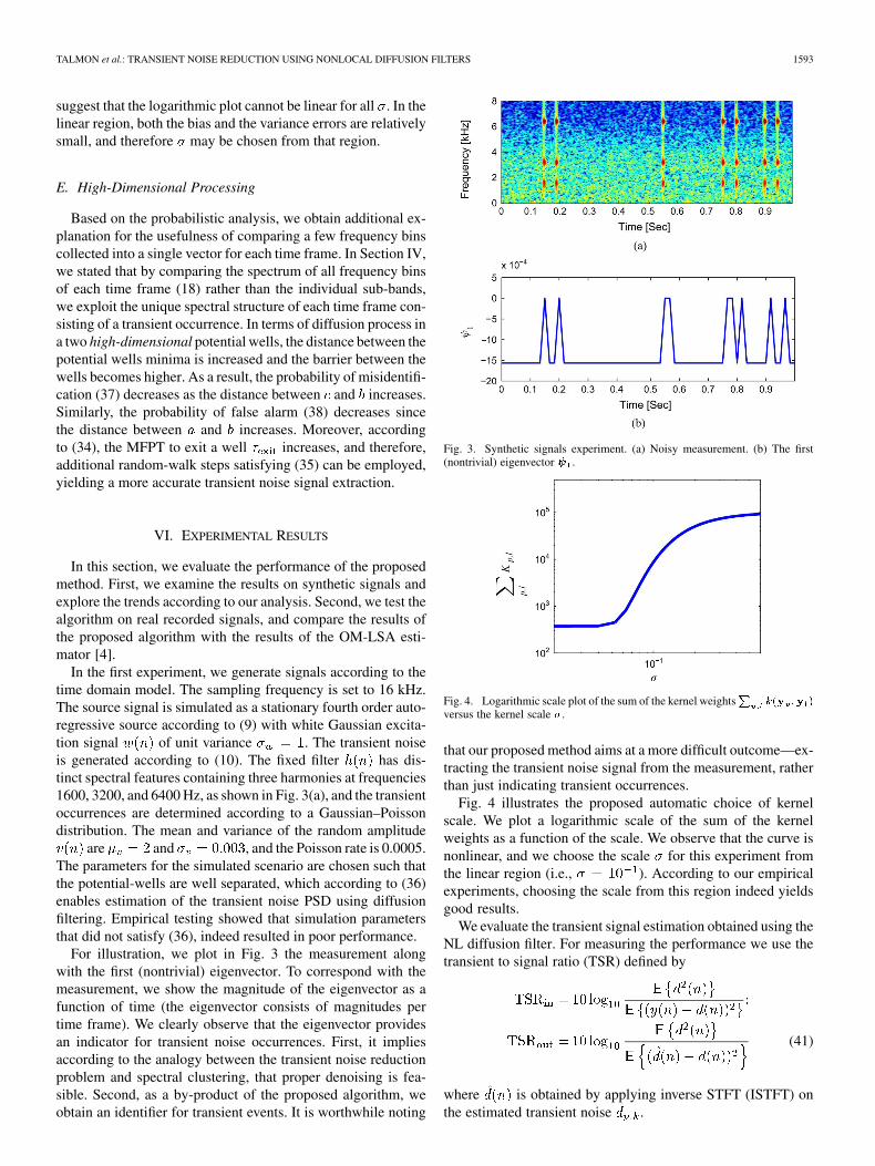
In the first experiment, we generate signals according to thetime domain model. The sampling frequency is set to 16 kHz.The source signal is simulated as a stationary fourth order auto-regressive source according to (9) with white Gaussian excita-tion signal of unit variance . The transient noiseis generated according to (10). The fixed filter has dis-tinct spectral features containing three harmonies at frequencies1600, 3200, and 6400 Hz, as shown in Fig. 3(a), and the transientoccurrences are determined according to a Gaussian–Poissondistribution. The mean and variance of the random amplitude

are and , and the Poisson rate is 0.0005.The parameters for the simulated scenario are chosen such thatthe potential-wells are well separated, which according to (36)enables estimation of the transient noise PSD using diffusionfiltering. Empirical testing showed that simulation parametersthat did not satisfy (36), indeed resulted in poor performance.

For illustration, we plot in Fig. 3 the measurement alongwith the first (nontrivial) eigenvector. To correspond with themeasurement, we show the magnitude of the eigenvector as afunction of time (the eigenvector consists of magnitudes pertime frame). We clearly observe that the eigenvector providesan indicator for transient noise occurrences. First, it impliesaccording to the analogy between the transient noise reductionproblem and spectral clustering, that proper denoising is fea-sible. Second, as a by-product of the proposed algorithm, weobtain an identifier for transient events. It is worthwhile noting

Fig. 3. Synthetic signals experiment. (a) Noisy measurement. (b) The first(nontrivial) eigenvector �� .

Fig. 4. Logarithmic scale plot of the sum of the kernel weights �� versus the kernel scale �.

that our proposed method aims at a more difficult outcome—ex-tracting the transient noise signal from the measurement, ratherthan just indicating transient occurrences.

Fig. 4 illustrates the proposed automatic choice of kernelscale. We plot a logarithmic scale of the sum of the kernelweights as a function of the scale. We observe that the curve isnonlinear, and we choose the scale for this experiment fromthe linear region (i.e., ). According to our empiricalexperiments, choosing the scale from this region indeed yieldsgood results.

We evaluate the transient signal estimation obtained using theNL diffusion filter. For measuring the performance we use thetransient to signal ratio (TSR) defined by

(41)

where is obtained by applying inverse STFT (ISTFT) onthe estimated transient noise .


Fig. 5. (a) TSR improvement (in dB) obtained as a function of the number of denoising steps. (b) Comparison of the obtained TSR improvement. (in dB) betweenlow and high transient occurrence divergence. (c) Comparison of the TSR improvement (in dB) between two different mean amplitude values.

Fig. 5(a) shows the TSR improvement obtained as a functionof the number of denoising steps. We note that in this experimentwe use powers of the transition matrix (the NL filter) , indi-cating several random-walk steps in each diffusion iteration. Weclearly observe the tradeoff in setting the proper number of stepsthat emerges from the results. Initially, we obtain an increase inthe TSR as we employ more steps. Then, after reaching a cer-tain number of steps (greater than the relaxation time), the TSRremains constant and applying more denoising steps does notimprove the results. Finally, when the number of steps reachesthe MFPT to exit a well, applying additional denoising stepssmears the signal, and the TSR decreases.

In Fig. 5(b), we compare the TSR improvement between lowand high transient occurrence divergence. For the low diver-gence case, we set the variance of the amplitude modulationin the simulation to be a small value , and for thehigh divergence case, we set in the simulation to be twicehigher. First, the TSR obtained when the transient occurrencesdivergence is high, is smaller than the TSR obtained when thedivergence is low. Since transient occurrences are less similar,the averaging obtained by the diffusion filter is less accuratesince the resulting mean value varies from each transient oc-currence. Second, we observe that in the high diversity case, weneed to apply more steps in order to reach optimal TSR values.However there is a sharp decline starting from smaller numberof iterations. By increasing the transient noise amplitude vari-ance, the potential well becomes wider, and the barrier lower.Consequently, the relaxation time of the right-hand well (corre-sponding to the transient occurrences) increases, and more dif-fusion steps should be used. In addition, the MFPT decreases,implying that less diffusion steps can be used.

Fig. 5(c) shows the obtained TSR improvement for two dif-ferent mean amplitude values (with the same vari-ance ). We observe that the TSR obtained when the mean am-plitude is small, is lower than the TSR obtained when the meanamplitude is large. In addition, a decay in the TSR occurs aftera smaller number of iterations, in the case of small mean ampli-tude. By decreasing the mean transient noise amplitude , thepotential wells become closer. As a consequence, the MFPT de-creases, and less diffusion steps can be used. In addition, sincethe separation of the two potential wells is worse, the probabilityfor misidentification increases.

In the second experiment, we use recorded speech and tran-sient noise signals. Speech signals sampled at 16 kHz are taken

Fig. 6. Signal spectrograms. (a) The noisy signal. (b) The whitened. signal�� .

from TIMIT database [42]. Various recorded transient noises aretaken from [43]. The measurements are constructed accordingto (7) and (8). The additive stationary noise part is a computergenerated white Gaussian noise with an SNR of 20 dB. Thelength of the speech utterance and the recorded transient noiseis 10 s. Such transient noise signal consists of 10 to 12 transientevents. We use short-time frames of 256 samples length bothfor the LPC estimation and for the STFT. The correspondingtime frame length is 16 ms, which is longer than the durationof the tested transients (approximately 10 ms). In each timeframe, we estimate AR envelope consisting of coef-ficients, in order to obtain a white excitation signal for bothvoiced and unvoiced phonemes (we verify that the pitch pe-riod is of shorter length). According to our empirical tests, sucha relatively short envelope enabled sufficient whitening of thespeech. Fig. 6 shows spectrograms of the noisy measurementwith metronome noise and the whitened signal . We ob-serve that the impulsive nature of transient events is maintained,while the speech phonemes are whitened. Specifically, we no-tice that AR coefficients provide satisfactory whiteningof both voiced and unvoiced phonemes to enable better distinc-tion of the transient events from the speech components.

The transient noise is extracted by the diffusion filter usingiterations. This specific number of iterations was


Fig. 7. Signal spectrograms. (a) The noisy signal. (b) The enhanced signal obtained by the OM-LSA. (c) The transient estimate obtained by the NL diffusionfilter. (d) The enhanced signal obtained by the proposed method.

Fig. 8. Signal spectrograms and waveforms in the area near the transient eventat 7.7 s. (a) The noisy signal. (b) The enhanced signal obtained by the proposedmethod.

chosen both according to the analysis from Section V alongwith empirical testing.

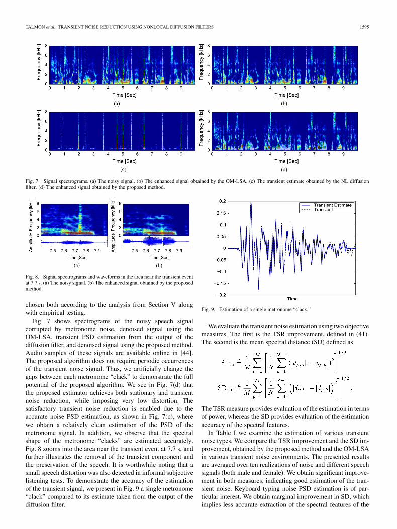
Fig. 7 shows spectrograms of the noisy speech signalcorrupted by metronome noise, denoised signal using theOM-LSA, transient PSD estimation from the output of thediffusion filter, and denoised signal using the proposed method.Audio samples of these signals are available online in [44].The proposed algorithm does not require periodic occurrencesof the transient noise signal. Thus, we artificially change thegaps between each metronome “clack” to demonstrate the fullpotential of the proposed algorithm. We see in Fig. 7(d) thatthe proposed estimator achieves both stationary and transientnoise reduction, while imposing very low distortion. Thesatisfactory transient noise reduction is enabled due to theaccurate noise PSD estimation, as shown in Fig. 7(c), wherewe obtain a relatively clean estimation of the PSD of themetronome signal. In addition, we observe that the spectralshape of the metronome “clacks” are estimated accurately.Fig. 8 zooms into the area near the transient event at 7.7 s, andfurther illustrates the removal of the transient component andthe preservation of the speech. It is worthwhile noting that asmall speech distortion was also detected in informal subjectivelistening tests. To demonstrate the accuracy of the estimationof the transient signal, we present in Fig. 9 a single metronome“clack” compared to its estimate taken from the output of thediffusion filter.

Fig. 9. Estimation of a single metronome “clack.”

We evaluate the transient noise estimation using two objectivemeasures. The first is the TSR improvement, defined in (41).The second is the mean spectral distance (SD) defined as

The TSR measure provides evaluation of the estimation in termsof power, whereas the SD provides evaluation of the estimationaccuracy of the spectral features.

In Table I we examine the estimation of various transientnoise types. We compare the TSR improvement and the SD im-provement, obtained by the proposed method and the OM-LSAin various transient noise environments. The presented resultsare averaged over ten realizations of noise and different speechsignals (both male and female). We obtain significant improve-ment in both measures, indicating good estimation of the tran-sient noise. Keyboard typing noise PSD estimation is of par-ticular interest. We obtain marginal improvement in SD, whichimplies less accurate extraction of the spectral features of the


TABLE IEVALUATION OF THE TRANSIENT SIGNAL ESTIMATION

transient noise. Due to the high divergence between transientoccurrences belonging to different key strokes, both in shapeand power, the averaging process results in a “mean tappingshape” which varies from the spectral shape of each individualkey press. Nevertheless, we observe good improvement in TSR,which indicates good estimation in terms of noise power. Sincethe potential-well associated with the excitation signal is wellseparated, the transient signal is properly extracted by the NLfilter, which enables accurate identification of transient eventstime locations, yielding significant reduction in the total noisepower at the output of the proposed algorithm. This particularnoise type demonstrates the robustness of the proposed algo-rithm. Even though the transient interference caused by key-board typing do not correspond to our assumptions, the pro-posed algorithm still enables improved result.

We evaluate the output of the proposed method using anothertwo objective measures. The first is the common signal to noiseratio, defined as

(42)

The second is the mean log spectral distance (LSD) between themeasured signal and the desired source, which is specificallyadapted to speech signals and defined as

where

and is a small value defined by , used toconfine the dynamic range of the log-spectrum to 50 dB.

To test the estimation of the speech in the presence of thetransient noise events, we present in Table II the results ob-tained only in time frames in (instead of the whole observa-tion interval). We compare the speech enhancement results ob-tained using the proposed method and the OM-LSA estimator.We present the two objective measures (SNR improvement andLSD improvement) in dB. We clearly observe that the proposedmethod achieves better results compared to the OM-LSA in allnoise types. It is worthwhile noting that similar results wereobtained for other transient noise types taken from [43]: roofhammering, door slams, household clacks, and other percussive

TABLE IIENHANCEMENT EVALUATION IN TRANSIENT OCCURRENCE PERIODS

noises. The results emphasize the advantage of the proposed al-gorithm in obtaining good transient noise reduction, while pre-serving speech components, even under the adverse conditionscreated by the presence of transient noise events.

VII. CONCLUSION

We have presented a novel approach for handling speech cor-rupted with transient interferences. The proposed approach isbased on the NL diffusion filter, that exploits the intrinsic geo-metric structure of the measurements. In particular, it relies onthe variation of speech components and sharp impulses of re-peating transient noise occurrences. By using diffusion interpre-tation of the NL filters, we gained insight into the behavior of theproposed method. Using the diffusion framework, we addressedthe problem of proper choice of parameters and evaluated theperformance and limitations of the proposed method. Experi-mental results have demonstrated that for repetitive and shorttransient occurrences, the proposed method obtains improvedresults, compared to those obtained by the OM-LSA estimator.In addition, the proposed method is robust to various types oftransient interferences.

The main component of the proposed algorithm is the esti-mation of the transient noise PSD using NL diffusion filtering.Here, we have incorporated the PSD estimate into the OM-LSAestimator for speech enhancement. However, the PSD estimatemay be exploited for other tasks as well. For example, it can beof major importance when developing a voice activity detector(VAD), adapted to transient noise environments. Future workwill address real-time implementation of the algorithm, and de-veloping a model for the spectral variations and durations ofthe transient events. For example, we aim at developing a morerobust algorithm based on two iterations of the NL filter. Thefirst iteration will provide just an estimate of the locations of thetransients. In the second iteration, given the transients locations,each transient amplitude, shape and duration will be estimatedand handled.

APPENDIX IGAUSSIAN NOISE EXAMPLE

We present a simple example of denoising a step function cor-rupted by Gaussian noise using NL filters. Let be adata set consisting of real samples . Each data sample,which consists of a desired constant corrupted by additive whiteGaussian noise, is given by

(43)

where are in with equal probability and areindependent and identically distributed Gaussian random vari-ables with zero mean and variance. For example,


Fig. 10. (a) Source signal. (b) The noisy measurement. (c) The denoised signalusing low-pass filter.

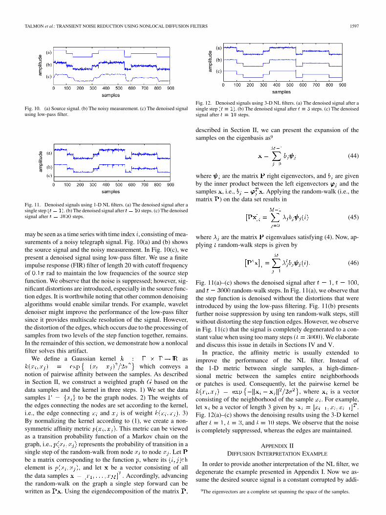
Fig. 11. Denoised signals using 1-D NL filters. (a) The denoised signal after asingle step �� . (b) The denoised signal after � � �� steps. (c) The denoisedsignal after � � �� steps.

may be seen as a time series with time index , consisting of mea-surements of a noisy telegraph signal. Fig. 10(a) and (b) showsthe source signal and the noisy measurement. In Fig. 10(c), wepresent a denoised signal using low-pass filter. We use a finiteimpulse response (FIR) filter of length 20 with cutoff frequencyof rad to maintain the low frequencies of the source stepfunction. We observe that the noise is suppressed; however, sig-nificant distortions are introduced, especially in the source func-tion edges. It is worthwhile noting that other common denoisingalgorithms would enable similar trends. For example, waveletdenoiser might improve the performance of the low-pass filtersince it provides multiscale resolution of the signal. However,the distortion of the edges, which occurs due to the processing ofsamples from two levels of the step function together, remains.In the remainder of this section, we demonstrate how a nonlocalfilter solves this artifact.

We define a Gaussian kernel aswhich conveys a

notion of pairwise affinity between the samples. As describedin Section II, we construct a weighted graph based on thedata samples and the kernel in three steps. 1) We set the datasamples to be the graph nodes. 2) The weights ofthe edges connecting the nodes are set according to the kernel,i.e., the edge connecting and is of weight . 3)By normalizing the kernel according to (1), we create a non-symmetric affinity metric . This metric can be viewedas a transition probability function of a Markov chain on thegraph, i.e., represents the probability of transition in asingle step of the random-walk from node to node . Letbe a matrix corresponding to the function , where itselement is , and let be a vector consisting of allthe data samples . Accordingly, advancingthe random-walk on the graph a single step forward can bewritten as . Using the eigendecomposition of the matrix ,

Fig. 12. Denoised signals using 3-D NL filters. (a) The denoised signal after asingle step �� . (b) The denoised signal after � � � steps. (c) The denoisedsignal after � � �� steps.

described in Section II, we can present the expansion of thesamples on the eigenbasis as9

(44)

where are the matrix right eigenvectors, and are givenby the inner product between the left eigenvectors and thesamples , i.e., . Applying the random-walk (i.e., thematrix ) on the data set results in

(45)

where are the matrix eigenvalues satisfying (4). Now, ap-plying random-walk steps is given by

(46)

Fig. 11(a)–(c) shows the denoised signal after , ,and random-walk steps. In Fig. 11(a), we observe thatthe step function is denoised without the distortions that wereintroduced by using the low-pass filtering. Fig. 11(b) presentsfurther noise suppression by using ten random-walk steps, stillwithout distorting the step function edges. However, we observein Fig. 11(c) that the signal is completely degenerated to a con-stant value when using too many steps . We elaborateand discuss this issue in details in Sections IV and V.

In practice, the affinity metric is usually extended toimprove the performance of the NL filter. Instead ofthe 1-D metric between single samples, a high-dimen-sional metric between the samples entire neighborhoodsor patches is used. Consequently, let the pairwise kernel be

, where is a vectorconsisting of the neighborhood of the sample . For example,let be a vector of length 3 given by .Fig. 12(a)–(c) shows the denoising results using the 3-D kernelafter , , and steps. We observe that the noiseis completely suppressed, whereas the edges are maintained.

APPENDIX IIDIFFUSION INTERPRETATION EXAMPLE

In order to provide another interpretation of the NL filter, wedegenerate the example presented in Appendix I. Now we as-sume the desired source signal is a constant corrupted by addi-

9The eigenvectors are a complete set spanning the space of the samples.


tive Gaussian noise, i.e., . In this case, from (43), we havethat the density of the samples is Gaussian

(47)

Thus, up to an additive constant, the potential, defined by, is parabolic

(48)

As shown in [24] and [25], for a large data setand small kernel scale , the transition matrix , whichrepresents the discrete random-walk on the graph, convergesto the continuous backward Fokker–Planck operator (6).When using scalars, we have that for every smooth function

, the resulting Fokker–Planck operator is merely asecond-order differential equation, given by

(49)

where and are first- and second-order derivatives of , andis the first derivative of the potential .

It can also be shown that the eigenvectors of are discreteapproximation of the eigenfunctions of . In our case, using (48)and (49), the eigenfunctions (which can be viewed as asmooth function on the data samples) satisfy the second-orderdifferential equation

(50)

where are the corresponding eigenvalues of the continuousFokker–Planck operator. The eigenfunctions that solve (50) areknown as the Hermite polynomials .The first three are given by , , and

. Thus, from (44) and the special form of theeigenfunction, we obtain that the expansion of the samples onthe eigenbasis consists of only the first two terms

(51)

where is a vectors of ones of length . Combining (46) and(51) yields

(52)

which means that each step of the random-walk shrinks thenoise in towards the desired mean value at rate . Con-sequently, we obtained that applying the random-walk on thedata set suppresses the additive Gaussian white noise and pro-vides an estimate of the desired constant.

ACKNOWLEDGMENT

The authors would like to thank Prof. Ronald Coifman forhelpful discussions. They also thank the anonymous reviewersfor their constructive comments and useful suggestions.

REFERENCES

[1] Y. Ephraim and D. Malah, “Speech enhancememt using a minimummean square error short time spectral amplitude estimator,” IEEETrans. Acoust., Speech, Signal Process., vol. 32, no. , pp. 1109–1121,Dec. 1984.

[2] Y. Ephraim and D. Malah, “Speech enhancement using a minimummean square error log spectral amplitude estimator,” IEEE Trans.Acoust., Speech, Signal Process., vol. 33, no. 2, pp. 443–445, Apr.1985.

[3] R. Martin, “Noise power spectral density estimation based on op-timal smoothing and minimum statistics,” IEEE Trans. Speech AudioProcess., vol. 9, no. 5, pp. 504–512, Jul. 2001.

[4] I. Cohen and B. Berdugo, “Speech enhancement for non-stationarynoise environments,” Signal Process., vol. 81, no. 11, pp. 2403–2418,Nov. 2001.

[5] I. Cohen and B. Berdugo, “Noise estimation by minima controlledrecursive averaging for robust speech enhancement,” IEEE SignalProcess. Lett., vol. 9, no. 1, pp. 12–15, Jan. 2002.

[6] I. Cohen, “Noise spectrum estimation in adverse environments: Im-proved minima controlled recursive averaging,” IEEE Trans. SpeechAudio Process., vol. 11, no. 5, pp. 466–475, Sep. 2003.

[7] S. V. Vaseghi and P. J. W. Rayner, “Detection and suppression ofimpulsive noise in speech communication systems,” IEE Proc. I:Commun. Speech Vis., pp. 38–46, Feb. 1990.

[8] S. Vaseghi, Advanced Digital Signal Processing and Noise Reduction,3rd ed. New York: Wiley, 2006.

[9] S. J. Godsill and P. J. W. Rayner, “Statistical reconstruction and anal-ysis of autoregressive signals in impulsive noise using the gibbs sam-pler,” IEEE Trans. Speech Audio Process., vol. 6, no. 4, pp. 352–372,Jul. 1998.

[10] L. P. Yaroslavski, Digital Picture Processing. Berlin, Germany:Springer-Verlag, 1985.

[11] D. Barash, “A fundamental relationship between bilateral filtering,adaptive smoothing, and the nonlinear diffusion equation,” IEEETrans. Pattern Anal. Mach. Intell., vol. 24, no. 6, pp. 844–847, Jun.2002.

[12] A. Buades, B. Coll, and J. M. Morel, “A review of image denoisingalgorithms, with a new one,” Multiscale Model. Simul., vol. 4, pp.490–530, 2005.

[13] M. Mahmoudi and G. Sapiro, “Fast image and video denoising via non-local means of similar neighborhoods,” IEEE Signal Process. Lett., vol.12, no. 12, pp. 839–842, Dec. 2005.

[14] A. D. Szlam, M. Maggioni, and R. Coifmain, “Regularization ongraphs with function-adapted diffusion processes,” J. Mach. Learn.Res., 2007.

[15] A. Singer, Y. Shkolnisky, and B. Nadler, “Diffusion interpretation ofnon local neighborhood filters for signal denoising,” SIAM J. ImagingSci., vol. 2, no. 1, pp. 118–139, 2009.

[16] A. Abramson and I. Cohen, “Enhancement of speech signals undermultiple hypotheses using an indicator for transient noise presence,” inProc. 32rd IEEE Int. Conf. Acoust. Speech Signal Process., ICASSP-2007, Honolulu, HI, Apr. 2007, pp. IV-553–556.

[17] R. Talmon, I. Cohen, and S. Gannot, “Speech enhancement in transientnoise environment using diffusion filtering,” in Proc. 35th IEEE Int.Conf. Acoust. Speech, Signal Process. (ICASSP’10), Dallas, TX, Mar.2010, pp. 4782–4785.

[18] B. Scholkopf, A. Smola, and K. Muller, “Nonlinear component anal-ysis as a kernel eigenvalue problem,” Neural Comput., vol. 10, pp.1299–1319, 1996.

[19] J. B. Tenenbaum, V. de Silva, and J. C. Langford, “A global geometricframework for nonlinear dimensionality reduction,” Science, vol. 260,pp. 2319–2323, 2000.

[20] S. T. Roweis and L. K. Saul, “Nonlinear dimensionality reduction bylocally linear embedding,” Science, vol. 260, pp. 2323–2326, 2000.

[21] M. Belkin and P. Niyogi, “Laplacian eigenmaps for dimensionalityreduction and data representation,” Neural Comput., vol. 15, pp.1373–1396, 2003.

[22] D. L. Donoho and C. Grimes, “Hessian eigenmaps: New locally linearembedding techniques for high-dimensional data,” Proc. Nat. Acad.Sci., vol. 100, pp. 5591–5596, 2003.

[23] R. Coifman, S. Lafon, A. B. Lee, M. Maggioni, B. Nadler, F. Warner,and S. W. Zucker, “Geometric diffusions as a tool for harmonic analysisand structure definition of data: Diffusion maps,” Proc. Nat. Acad. Sci.,vol. 102, no. 21, pp. 7426–7431, May 2005.

[24] R. Coifman and S. Lafon, “Diffusion maps,” Appl. Comput. Harmon.Anal., vol. 21, pp. 5–30, Jul. 2006.


[25] B. Nadler, S. Lafon, R. Coifman, and I. G. Kevrekidis, “Diffusion maps,spectral clustering and reaction coordinates of dynamical systems,”Appl. Comput. Harmon. Anal., pp. 113–127, 2006.

[26] F. R. K. Chung, Spectral Graph Theory, 1997, CBMS-AMS.[27] G. W. Gardiner, Handbook of Stochastic Processes for Physics, 2nd

ed. Berlin, Germany: Springer-Verlag, 2002.[28] B. J. Matkowsky and Z. Schuss, “Eigenvalues of the Fokker-Planck op-

erator and the approach to equilibrium for diffusions in potential fields,”SIAM J. Appl. Math., vol. 40, pp. 242–254, 1981.

[29] B. Nadler, S. Lafon, R. Coifman, and I. G. Kevrekidis, “Diffusionmaps, spectral clustering and eigenfunctions of Fokker-Planck opera-tors,” Neural Inf. Process. Syst. (NIPS), vol. 18, 2005.

[30] B. Nadler and M. Galun, “Fundamental limitations of spectral clus-tering,” Neural Inf. Process. Syst. (NIPS), vol. 19, 2006.

[31] T. F. Quatieri, Discrete Time Speech Signal Processing Principles andPractice. Englewood Cliffs, NJ: Prentice-Hall, 2001.

[32] S. Godsill, Digital Audio Restoration—A Statistical Model Based Ap-proach. London, U.K.: Springer-Verlag, 1998.

[33] Y. Avargel and I. Cohen, “On multiplicative transfer function approx-imation in the short time Fourier transform domain,” IEEE SignalProcess. Lett., vol. 14, no. 5, pp. 337–340, May 2007.

[34] M. Belkin and P. Niyogi, “Convergence of Laplacian Eigenmaps,” inAdvances in Neural Information Processing Systems (NIPS) 19, B.Schölkopf and T. Hoffman, Eds. Cambridge, MA: MIT Press, 2007,pp. 129–136.

[35] Y. Weiss, “Segmentation using eigenvectors: A unifying view,” in Proc.Int. Conf. Comput. Vis., 1999.

[36] J. Shi and J. Malik, “Normalized cuts and image segmentation,” IEEETrans. Pattern Anal. Mach. Intell., vol. 22, no. 8, pp. 888–905, Aug.2000.

[37] M. Meila and J. Shi, “A random walks view of spectral segmentation,”in 8th Int. Workshop Artif. Intell. Statist., 2001.

[38] A. Y. Ng, M. Jordan, and Y. Weiss, “On spectral clustering: Anal-ysis and an algorithm,” in Advances in Neural Information ProcessingSystems, T. G. Dietterich, S. Becker, and Z. Ghahramani, Eds. Cam-bridge, MA: MIT Press, 2002, pp. 849–856.

[39] M. Hein and J. Y. Audibert, L. De Raedt and S. Wrobel, Eds., “Intrinsicdimensionality estimation of submanifold in � ,” in Proc. 22nd Int.Conf. Mach. Learn., ACM, 2005, pp. 289–296.

[40] A. Singer, “From graph to manifold Laplacian: The convergence rate,”Appl. Comput. Harmon. Anal., vol. 21, pp. 128–134, 2006.

[41] R. R. Coifman, Y. Shkolnisky, F. J. Sigworth, and A. Singer, “GraphLaplacian tomography from unknown random projections,” IEEETrans. Image Process., vol. 17, no. 10, pp. 1891–1899, Oct. 2008.

[42] J. S. Garofolo, “Getting Started With the DARPA TIMIT CD-ROM:An Acoustic-Phonetic Continous Speech Database,” Nat. Inst. of Stan-dards and Technology (NIST), Gaithersburg, MD, 1993.

[43] [Online]. Available: http://www.freesound.org[44] [Online]. Available: http://www.eng.biu.ac.il/~gannot/

Ronen Talmon (S’09) received the B.A degree inmathematics and computer science from the OpenUniversity, Ra’anana, Israel, in 2005. He is currentlypursuing the Ph.D. degree in electrical engineering atthe Technion—Israel Institute of Technology, Haifa.

From 2000 to 2005, he was a Software Developerand Researcher in a technological unit of the IsraeliDefense Forces. Since 2005, he has been a TeachingAssistant and a Project Supervisor with the Signaland Image Processing Lab (SIPL), Electrical Engi-neering Department, Technion. His research interests

are statistical signal processing, speech enhancement, system identification, har-monic analysis, and geometric methods for data analysis.

Israel Cohen (M’01–SM’03) received the B.Sc.(summa cum laude), M.Sc., and Ph.D. degrees inelectrical engineering from the Technion-IsraelInstitute of Technology, Haifa, in 1990, 1993, and1998, respectively.

From 1990 to 1998, he was a Research Scientistwith RAFAEL Research Laboratories, Haifa, Israel,Ministry of Defense. From 1998 to 2001, he was aPostdoctoral Research Associate with the ComputerScience Department, Yale University, New Haven,CT. In 2001, he joined the Electrical Engineering

Department, Technion, where he is currently an Associate Professor. Hisresearch interests are statistical signal processing, analysis and modeling ofacoustic signals, speech enhancement, noise estimation, microphone arrays,source localization, blind source separation, system identification, and adaptivefiltering. He is a coeditor of the Multichannel Speech Processing section ofthe Springer Handbook of Speech Processing (Springer, 2008), a coauthor ofNoise Reduction in Speech Processing (Springer, 2009), a coeditor of SpeechProcessing in Modern Communication: Challenges and Perspectives (Springer,2010), and a cochair of the 2010 International Workshop on Acoustic Echo andNoise Control.

Dr. Cohen is a recipient of the Alexander Goldberg Prize for Excellence inResearch and the Muriel and David Jacknow Award for Excellence in Teaching.He served as Associate Editor of the IEEE TRANSACTIONS ON AUDIO, SPEECH,AND LANGUAGE PROCESSING and IEEE SIGNAL PROCESSING LETTERS, and asGuest Editor of a special issue of the EURASIP Journal on Advances in SignalProcessing on Advances in Multimicrophone Speech Processing and a specialissue of the EURASIP Speech Communication Journal on Speech Enhancement.

Sharon Gannot (S’92–M’01–SM’06) received theB.Sc. degree (summa cum laude) from the Tech-nion-Israel Institute of Technology, Haifa, in 1986and the M.Sc. (cum laude) and Ph.D. degrees fromTel-Aviv University, Tel-Aviv, Israel, in 1995 and2000, respectively, all in electrical engineering.

In 2001, he held a post-doctoral position at theDepartment of Electrical Engineering (SISTA),K.U.Leuven, Leuven, Belgium. From 2002 to 2003,he held a research and teaching position at the Fac-ulty of Electrical Engineering, Technion. Currently,

he is an Associate Professor in the School of Engineering, Bar-Ilan University,Ramat-Gan, Israel.

Dr. Gannot is the recipient of Bar-Ilan University Outstanding LecturerAward for the year 2010. He is an Associate Editor of the IEEE TRANSACTIONS

ON AUDIO, SPEECH, AND LANGUAGE PROCESSING, and a member of theIEEE Audio and Acoustic Signal Processing Technical Committee. He is alsoAssociate Editor of the EURASIP Journal on Advances in Signal Processing,an Editor of two special issues on Multi-Microphone Speech Processing of thesame journal, a guest editor of the ELSEVIER Speech Communication journaland a reviewer of many IEEE journals and conferences. He has been a memberof the Technical and Steering Committee of the International Workshop onAcoustic Echo and Noise Control (IWAENC) since 2005 and the generalco-chair of IWAENC 2010 held in Tel-Aviv. His research interests includeparameter estimation, statistical signal processing, and speech processing usingeither single- or multi-microphone arrays.

Documents

1584 IEEE TRANSACTIONS ON AUDIO, SPEECH, AND LANGUAGE ... · 1584 IEEE TRANSACTIONS ON AUDIO, SPEECH, AND LANGUAGE PROCESSING, VOL. 19, NO. 6, AUGUST 2011 Transient Noise Reduction