148 Chapter 6 Chapter 6 - westada.org

Chapter 6 6.1 Answers will vary but examples are: (a) Flip the coin twice. Let HH represent a failure, and let the other three outcomes, HT, TH, TT, represent a success. (b) Let 1, 2, and 3 represent a success, and let 4 represent a failure. If 5 or 6 come up, ignore them and roll again. (c) Peel off two consecutive digits from the table; let 00 through 74 represent a success, and let 75 through 99 represent a failure. (d) Let diamonds, spades, clubs represent a success, and let hearts represent a failure. You must replace the card and shuffle the deck before the next trial to maintain independence. 6.2 Flip both nickels at the same time. Let HH represent a success (the occurrence of the phenomenon of interest) and HT, TH, TT represent a failure (the nonoccurrence of the phenomenon). 6.3 (a) Obtain an alphabetical list of the student body, and assign consecutive numbers to the students on the list. Use a random process (table or random digit generator) to select 10 students from this list. (b) Let the two-digit groups 00 to 83 represent a “Yes” to the question of whether or not to abolish evening exams and the groups 84 to 99 represent a “No.” (c) Starting at line 129 in Table B (“Yes” in boldface) and moving across rows:

Repetition 1: 36, 75, 95, 89, 84, 68, 28, 82, 29, 13 # “Yes”: 7. Repetition 2: 18, 63, 85, 43, 03, 00, 79, 50, 87, 27 # “Yes”: 8. Repetition 3: 69, 05, 16, 48, 17, 87, 17, 40, 95, 17 # “Yes”: 8. Repetition 4: 84, 53, 40, 64, 89, 87, 20, 19, 72, 45 # “Yes”: 7. Repetition 5: 05, 00, 71, 66, 32, 81, 19, 41, 48, 73 # “Yes”: 10.

(Theoretically, we should achieve 10 “Yes” results approximately 17.5% of the time.) 6.4 (a) A single random digit simulates one shot, with 0 to 6 representing a made basket and 7, 8, or 9 representing a miss. Then 5 consecutive digits simulate 5 independent shots. (b) Let 0–6 represent a “made basket” and 7, 8, 9 represent a “missed basket.” Starting with line 125, the first four repetitions are:

Repetition 9 6 7 4 6 1 2 1 4 9 3 7 8 2 3 7 1 8 6 8 Number of misses (2) (1) (2) (3)

Each block of 5 digits in the table represents one repetition of the 5 attempted free throws. The underlined digits represent made baskets. We perform 46 more repetitions for a total of 50, and calculate the relative frequency that a player misses 3 or more of 5 shots. Here are the numbers of baskets missed for the 50 repetitions.

2 1 2 3 1 1 0 1 3 2 2 2 3 3 2 1 2 4 0 1 1 1 2 1 2 1 0 1 0 2 3 3 2 3 3 1 2 0 2 3 1 2 3 2 1 2 2 2 1 0

A frequency table for the number of missed shots is shown below. Number of misses 0 1 2 3 4 5Frequency 6 15 18 10 1 0

The relative frequency of missing 3 or more shots in 5 attempts is 11/50 = 0.22. Note: The theoretical probability of missing 3 or more shots is 0.1631.

148 Chapter 6

6.5 The choice of digits in these simulations may of course vary from that made here. In (a)–(c), a single digit simulates the response; for (d), two digits simulate the response of a single voter. (a) Odd digits represent a Democratic choice; even digits represent a Republican choice. (b) 0, 1, 2, 3, 4, 5 represent a Democratic choice and 6, 7, 8, 9 represent a Republican choice. (c) 0, 1, 2, 3 represent a Democratic choice; 4, 5, 6, 7 represent a Republican choice; 8, 9 represent Undecided. (d) 00, 01,…, 52 represent a Democratic choice and 53, 54,…, 99 represent a Republican choice. 6.6 For the choices made in the solution to Exercise 6.5: (a) D, R, R, R, R, R, R, D, R, D — 3 Democrats, 7 Republicans (b) R, D, D, R, R, R, R, D, R, R — 3 Democrats, 7 Republicans (c) R, U, R, D, R, U, U, U, D, R — 2 Democrats, 4 Republicans, 4 undecided (d) R, R, R, D, D, D, D, D, D, R — 6 Democrats, 4 Republicans 6.7 Let 1 represent a girl and 0 represent a boy. The command randInt(0,1,4) produces a 0 or 1 with equal likelihood in groups of 4. Continue to press ENTER. In 50 repetitions, we got at least one girl 47 times, and no girls three times. Our simulation produced a girl 94% of the time, vs. a probability of 0.938 obtained in Example 6.6. 6.8 (a) Let the digits 0, 1, 2, 3, 4, 5 correspond to the American League team winning a Series game and 6, 7, 8, 9 correspond to the National League team winning. Single digits are chosen until one team has won four games, with a minimum of four digits and a maximum of seven digits being chosen. On the TI-83, you can use the command randInt (0, 9, 1) repeatedly to generate the digits. Here are two repetitions:

0, 3, 9, 2, 7, 9, 2 AL, AL, NL, AL, NL, NL, AL # games = 7 3, 0, 9, 1, 0 AL, AL, NL, AL, AL # games = 5

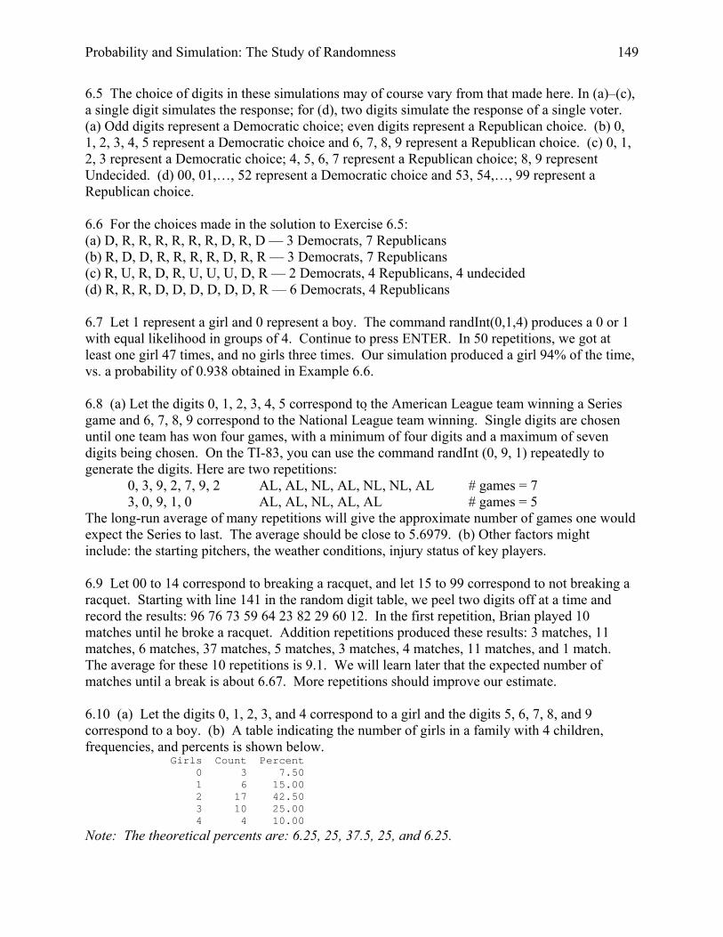
The long-run average of many repetitions will give the approximate number of games one would expect the Series to last. The average should be close to 5.6979. (b) Other factors might include: the starting pitchers, the weather conditions, injury status of key players. 6.9 Let 00 to 14 correspond to breaking a racquet, and let 15 to 99 correspond to not breaking a racquet. Starting with line 141 in the random digit table, we peel two digits off at a time and record the results: 96 76 73 59 64 23 82 29 60 12. In the first repetition, Brian played 10 matches until he broke a racquet. Addition repetitions produced these results: 3 matches, 11 matches, 6 matches, 37 matches, 5 matches, 3 matches, 4 matches, 11 matches, and 1 match. The average for these 10 repetitions is 9.1. We will learn later that the expected number of matches until a break is about 6.67. More repetitions should improve our estimate. 6.10 (a) Let the digits 0, 1, 2, 3, and 4 correspond to a girl and the digits 5, 6, 7, 8, and 9 correspond to a boy. (b) A table indicating the number of girls in a family with 4 children, frequencies, and percents is shown below.

Girls Count Percent 0 3 7.50 1 6 15.00 2 17 42.50 3 10 25.00 4 4 10.00

Note: The theoretical percents are: 6.25, 25, 37.5, 25, and 6.25.

Probability and Simulation: The Study of Randomness 149

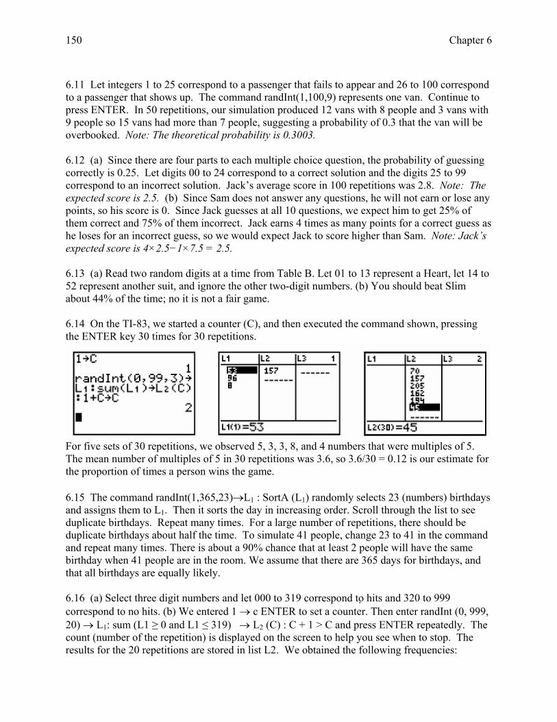
6.11 Let integers 1 to 25 correspond to a passenger that fails to appear and 26 to 100 correspond to a passenger that shows up. The command randInt(1,100,9) represents one van. Continue to press ENTER. In 50 repetitions, our simulation produced 12 vans with 8 people and 3 vans with 9 people so 15 vans had more than 7 people, suggesting a probability of 0.3 that the van will be overbooked. Note: The theoretical probability is 0.3003. 6.12 (a) Since there are four parts to each multiple choice question, the probability of guessing correctly is 0.25. Let digits 00 to 24 correspond to a correct solution and the digits 25 to 99 correspond to an incorrect solution. Jack’s average score in 100 repetitions was 2.8. Note: The expected score is 2.5. (b) Since Sam does not answer any questions, he will not earn or lose any points, so his score is 0. Since Jack guesses at all 10 questions, we expect him to get 25% of them correct and 75% of them incorrect. Jack earns 4 times as many points for a correct guess as he loses for an incorrect guess, so we would expect Jack to score higher than Sam. Note: Jack’s expected score is 4×2.5−1×7.5 = 2.5. 6.13 (a) Read two random digits at a time from Table B. Let 01 to 13 represent a Heart, let 14 to 52 represent another suit, and ignore the other two-digit numbers. (b) You should beat Slim about 44% of the time; no it is not a fair game. 6.14 On the TI-83, we started a counter (C), and then executed the command shown, pressing the ENTER key 30 times for 30 repetitions.

For five sets of 30 repetitions, we observed 5, 3, 3, 8, and 4 numbers that were multiples of 5. The mean number of multiples of 5 in 30 repetitions was 3.6, so 3.6/30 = 0.12 is our estimate for the proportion of times a person wins the game. 6.15 The command randInt(1,365,23)→L1 : SortA (L1) randomly selects 23 (numbers) birthdays and assigns them to L1. Then it sorts the day in increasing order. Scroll through the list to see duplicate birthdays. Repeat many times. For a large number of repetitions, there should be duplicate birthdays about half the time. To simulate 41 people, change 23 to 41 in the command and repeat many times. There is about a 90% chance that at least 2 people will have the same birthday when 41 people are in the room. We assume that there are 365 days for birthdays, and that all birthdays are equally likely. 6.16 (a) Select three digit numbers and let 000 to 319 correspond to hits and 320 to 999 correspond to no hits. (b) We entered 1 → c ENTER to set a counter. Then enter randInt (0, 999, 20) → L1: sum (L1 ≥ 0 and L1 ≤ 319) → L2 (C) : C + 1 > C and press ENTER repeatedly. The count (number of the repetition) is displayed on the screen to help you see when to stop. The results for the 20 repetitions are stored in list L2. We obtained the following frequencies:

150 Chapter 6

Number of hits in 20 at bats 4 5 6 7 8 9 Frequency 3 5 4 3 2 3

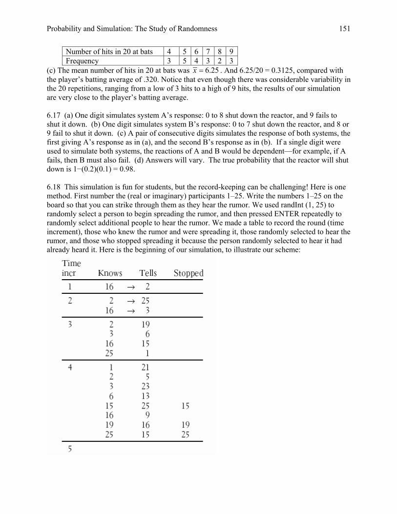
(c) The mean number of hits in 20 at bats was 6.25x = . And 6.25/20 = 0.3125, compared with the player’s batting average of .320. Notice that even though there was considerable variability in the 20 repetitions, ranging from a low of 3 hits to a high of 9 hits, the results of our simulation are very close to the player’s batting average. 6.17 (a) One digit simulates system A’s response: 0 to 8 shut down the reactor, and 9 fails to shut it down. (b) One digit simulates system B’s response: 0 to 7 shut down the reactor, and 8 or 9 fail to shut it down. (c) A pair of consecutive digits simulates the response of both systems, the first giving A’s response as in (a), and the second B’s response as in (b). If a single digit were used to simulate both systems, the reactions of A and B would be dependent—for example, if A fails, then B must also fail. (d) Answers will vary. The true probability that the reactor will shut down is 1−(0.2)(0.1) = 0.98. 6.18 This simulation is fun for students, but the record-keeping can be challenging! Here is one method. First number the (real or imaginary) participants 1–25. Write the numbers 1–25 on the board so that you can strike through them as they hear the rumor. We used randInt (1, 25) to randomly select a person to begin spreading the rumor, and then pressed ENTER repeatedly to randomly select additional people to hear the rumor. We made a table to record the round (time increment), those who knew the rumor and were spreading it, those randomly selected to hear the rumor, and those who stopped spreading it because the person randomly selected to hear it had already heard it. Here is the beginning of our simulation, to illustrate our scheme:


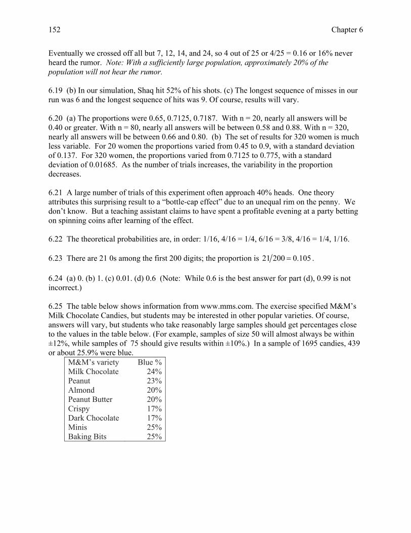
Eventually we crossed off all but 7, 12, 14, and 24, so 4 out of 25 or 4/25 = 0.16 or 16% never heard the rumor. Note: With a sufficiently large population, approximately 20% of the population will not hear the rumor. 6.19 (b) In our simulation, Shaq hit 52% of his shots. (c) The longest sequence of misses in our run was 6 and the longest sequence of hits was 9. Of course, results will vary. 6.20 (a) The proportions were 0.65, 0.7125, 0.7187. With n = 20, nearly all answers will be 0.40 or greater. With n = 80, nearly all answers will be between 0.58 and 0.88. With n = 320, nearly all answers will be between 0.66 and 0.80. (b) The set of results for 320 women is much less variable. For 20 women the proportions varied from 0.45 to 0.9, with a standard deviation of 0.137. For 320 women, the proportions varied from 0.7125 to 0.775, with a standard deviation of 0.01685. As the number of trials increases, the variability in the proportion decreases. 6.21 A large number of trials of this experiment often approach 40% heads. One theory attributes this surprising result to a “bottle-cap effect” due to an unequal rim on the penny. We don’t know. But a teaching assistant claims to have spent a profitable evening at a party betting on spinning coins after learning of the effect. 6.22 The theoretical probabilities are, in order: 1/16, 4/16 = 1/4, 6/16 = 3/8, 4/16 = 1/4, 1/16. 6.23 There are 21 0s among the first 200 digits; the proportion is 21 200 0.105= . 6.24 (a) 0. (b) 1. (c) 0.01. (d) 0.6 (Note: While 0.6 is the best answer for part (d), 0.99 is not incorrect.) 6.25 The table below shows information from www.mms.com. The exercise specified M&M’s Milk Chocolate Candies, but students may be interested in other popular varieties. Of course, answers will vary, but students who take reasonably large samples should get percentages close to the values in the table below. (For example, samples of size 50 will almost always be within ±12%, while samples of 75 should give results within ±10%.) In a sample of 1695 candies, 439 or about 25.9% were blue.

M&M’s variety Blue % Milk Chocolate 24% Peanut 23% Almond 20% Peanut Butter 20% Crispy 17% Dark Chocolate 17% Minis 25% Baking Bits 25%

152 Chapter 6

6.26 (a) We expect probability 1/2 (for the first flip, or for any flip of the coin). (b) The theoretical probability that the first head appears on an odd-numbered toss of a fair coin is

3 51 1 12 2 2

⎛ ⎞ ⎛ ⎞+ + + =⎜ ⎟ ⎜ ⎟⎝ ⎠ ⎝ ⎠

… 23

. Most answers should be between about 0.47 and 0.87.

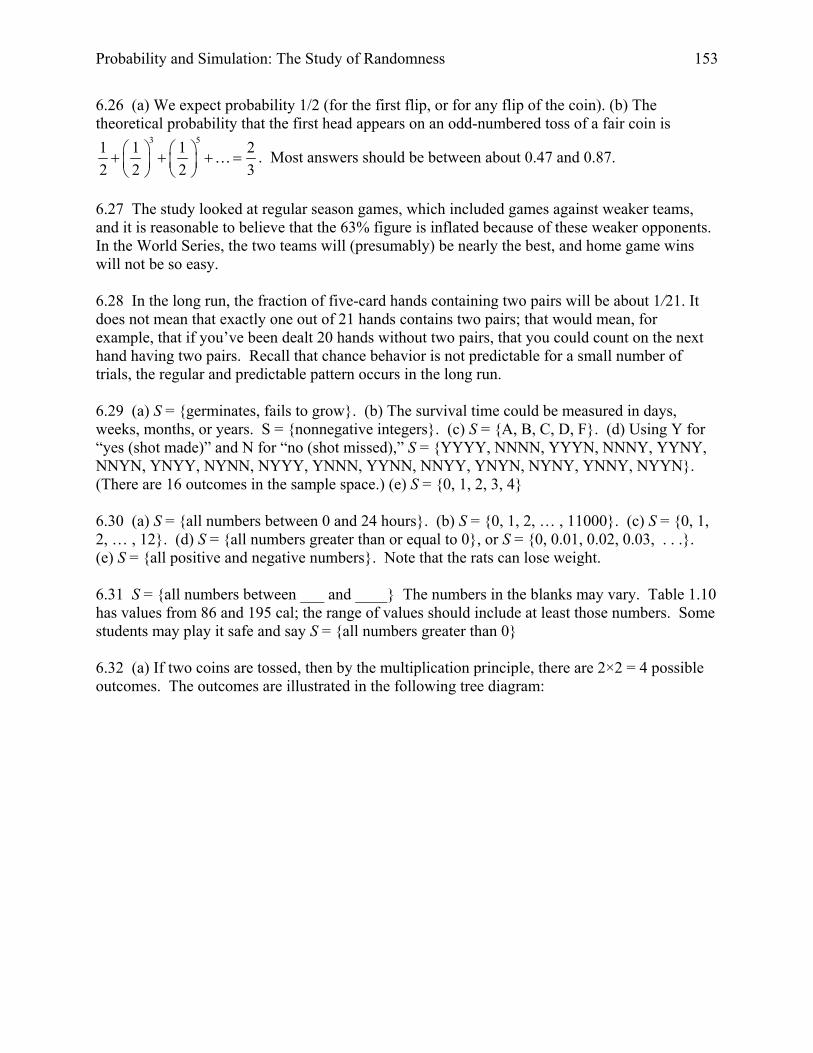
6.27 The study looked at regular season games, which included games against weaker teams, and it is reasonable to believe that the 63% figure is inflated because of these weaker opponents. In the World Series, the two teams will (presumably) be nearly the best, and home game wins will not be so easy. 6.28 In the long run, the fraction of five-card hands containing two pairs will be about 1/21. It does not mean that exactly one out of 21 hands contains two pairs; that would mean, for example, that if you’ve been dealt 20 hands without two pairs, that you could count on the next hand having two pairs. Recall that chance behavior is not predictable for a small number of trials, the regular and predictable pattern occurs in the long run. 6.29 (a) S = {germinates, fails to grow}. (b) The survival time could be measured in days, weeks, months, or years. S = {nonnegative integers}. (c) S = {A, B, C, D, F}. (d) Using Y for “yes (shot made)” and N for “no (shot missed),” S = {YYYY, NNNN, YYYN, NNNY, YYNY, NNYN, YNYY, NYNN, NYYY, YNNN, YYNN, NNYY, YNYN, NYNY, YNNY, NYYN}. (There are 16 outcomes in the sample space.) (e) S = {0, 1, 2, 3, 4} 6.30 (a) S = {all numbers between 0 and 24 hours}. (b) S = {0, 1, 2, … , 11000}. (c) S = {0, 1, 2, … , 12}. (d) S = {all numbers greater than or equal to 0}, or S = {0, 0.01, 0.02, 0.03, . . .}. (e) S = {all positive and negative numbers}. Note that the rats can lose weight. 6.31 S = {all numbers between ___ and ____} The numbers in the blanks may vary. Table 1.10 has values from 86 and 195 cal; the range of values should include at least those numbers. Some students may play it safe and say S = {all numbers greater than 0} 6.32 (a) If two coins are tossed, then by the multiplication principle, there are 2×2 = 4 possible outcomes. The outcomes are illustrated in the following tree diagram:


Start

H

T

H

T

H

T

HH

TT

TH

HT

Toss 2Toss 1

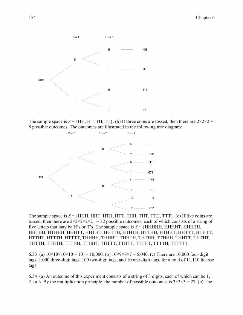
The sample space is S = {HH, HT, TH, TT}. (b) If three coins are tossed, then there are 2×2×2 = 8 possible outcomes. The outcomes are illustrated in the following tree diagram:

The sample space is S = {HHH, HHT, HTH, HTT, THH, THT, TTH, TTT}. (c) If five coins are tossed, then there are 2×2×2×2×2 = 32 possible outcomes, each of which consists of a string of five letters that may be H’s or T’s. The sample space is S = {HHHHH, HHHHT, HHHTH, HHTHH, HTHHH, HHHTT, HHTHT, HHTTH, HTHTH, HTTHH, HTHHT, HHTTT, HTHTT, HTTHT, HTTTH, HTTTT, THHHH, THHHT, THHTH, THTHH, TTHHH, THHTT, THTHT, THTTH, TTHTH, TTTHH, TTHHT, THTTT, TTHTT, TTTHT, TTTTH, TTTTT}. 6.33 (a) 10×10×10×10 = 104 = 10,000. (b) 10×9×8×7 = 5,040. (c) There are 10,000 four-digit tags, 1,000 three-digit tags, 100 two-digit tags, and 10 one-digit tags, for a total of 11,110 license tags. 6.34 (a) An outcome of this experiment consists of a string of 3 digits, each of which can be 1, 2, or 3. By the multiplication principle, the number of possible outcomes is 3×3×3 = 27. (b) The

154 Chapter 6

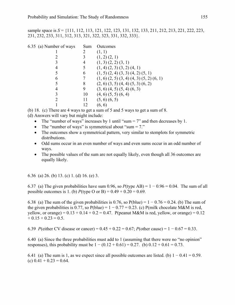
sample space is S = {111, 112, 113, 121, 122, 123, 131, 132, 133, 211, 212, 213, 221, 222, 223, 231, 232, 233, 311, 312, 313, 321, 322, 323, 331, 332, 333}. 6.35 (a) Number of ways Sum Outcomes

1 2 (1, 1) 2 3 (1, 2) (2, 1) 3 4 (1, 3) (2, 2) (3, 1) 4 5 (1, 4) (2, 3) (3, 2) (4, 1) 5 6 (1, 5) (2, 4) (3, 3) (4, 2) (5, 1) 6 7 (1, 6) (2, 5) (3, 4) (4, 3) (5, 2) (6, 1) 5 8 (2, 6) (3, 5) (4, 4) (5, 3) (6, 2) 4 9 (3, 6) (4, 5) (5, 4) (6, 3) 3 10 (4, 6) (5, 5) (6, 4) 2 11 (5, 6) (6, 5) 1 12 (6, 6)

(b) 18. (c) There are 4 ways to get a sum of 5 and 5 ways to get a sum of 8. (d) Answers will vary but might include:

• The “number of ways” increases by 1 until “sum = 7” and then decreases by 1. • The “number of ways” is symmetrical about “sum = 7.” • The outcomes show a symmetrical pattern, very similar to stemplots for symmetric

distributions. • Odd sums occur in an even number of ways and even sums occur in an odd number of

ways. • The possible values of the sum are not equally likely, even though all 36 outcomes are

equally likely. 6.36 (a) 26. (b) 13. (c) 1. (d) 16. (e) 3. 6.37 (a) The given probabilities have sum 0.96, so P(type AB) = 1 − 0.96 = 0.04. The sum of all possible outcomes is 1. (b) P(type O or B) = 0.49 + 0.20 = 0.69. 6.38 (a) The sum of the given probabilities is 0.76, so P(blue) = 1 − 0.76 = 0.24. (b) The sum of the given probabilities is 0.77, so P(blue) = 1 − 0.77 = 0.23. (c) P(milk chocolate M&M is red, yellow, or orange) = 0.13 + 0.14 + 0.2 = 0.47. P(peanut M&M is red, yellow, or orange) = 0.12 + 0.15 + 0.23 = 0.5. 6.39 P(either CV disease or cancer) = 0.45 + 0.22 = 0.67; P(other cause) = 1 − 0.67 = 0.33. 6.40 (a) Since the three probabilities must add to 1 (assuming that there were no “no opinion” responses), this probability must be 1 − (0.12 + 0.61) = 0.27. (b) 0.12 + 0.61 = 0.73. 6.41 (a) The sum is 1, as we expect since all possible outcomes are listed. (b) 1 − 0.41 = 0.59. (c) 0.41 + 0.23 = 0.64.


6.42 There are 19 outcomes where at least one digit occurs in the correct position: 111, 112, 113, 121, 122, 123, 131, 132, 133, 213, 221, 222, 223, 233, 313, 321, 322, 323, 333. The theoretical probability of at least one digit occurring in the correct position is therefore 19/27 = 0.7037. 6.43 (a) The table below gives the probabilities for the number of spots on the down-face when tossing a balanced (or “fair”) 4-sided die.

Number of spots 1 2 3 4 Probability 0.25 0.25 0.25 0.25

Since all 4 faces have the same shape and the same area, it is reasonable to assume that any one of the 4 faces is equally likely to be the down-face. Since the sum of the probabilities must be one, the probability of each should be 0.25. (b) The possible outcomes are (1,1) (1,2) (1,3) (1,4) (2,1) (2,2) (2,3) (2,4) (3,1) (3,2) (3,3) (3,4) (4,1) (4,2) (4,3) (4,4). The probability of any pair is 1/16 = 0.0625. The table below gives the probabilities for the sum of the number of spots on the down-faces when tossing two balanced (or “fair”) 4-sided dice.

Sum of spots 2 3 4 5 6 7 8 Probability 1/16 2/16 3/16 4/16 3/16 2/16 1/16

P(Sum = 5) = P(1,4) + P(2,3) + P(3,2) + P(4,1) = (0.0625) (4) = 0.25. 6.44 (a) P(D) = P(1, 2, or 3) = 0.301 + 0.176 + 0.125 = 0.602. (b) ( )P B D∪ = P(B) + P(D) =

0.602 + 0.222 = 0.824. (c) P(Dc) = 1 − P(D) = 1 − 0.602 = 0.398. (d) ( )P C D∩ = P(1 or 3) = 0.301 + 0.125 = 0.426. (e) = P(7 or 9) = 0.058 + 0.046 = 0.104. (P B C∩ ) 6.45 Fight one big battle: His probability of winning is 0.6, which is higher than the probability 0.83 = 0.512 of winning all three small battles. 6.46 The probability that all 12 chips in a car will work is ( ) . ( )12 121 0.05 0.95 0.5404− = 6.47 No: It is unlikely that these events are independent. In particular, it is reasonable to expect that college graduates are less likely to be laborers or operators.

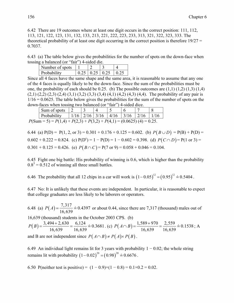
6.48 (a) ( ) 7,317 0.439716,639

P A = or about 0.44, since there are 7,317 (thousand) males out of

16,639 (thousand) students in the October 2003 CPS. (b)

( ) 3,494 2,630 6,124 0.368116,639 16,639

P B += = . (c) ( ) 1,589 970 2,559 0.1538

16,639 16,639P A B +

∩ = = ; A

and B are not independent since ( ) ( ) ( )P A B P A P B∩ ≠ × . 6.49 An individual light remains lit for 3 years with probability 1 − 0.02; the whole string remains lit with probability ( ) . ( )20 201 0.02 0.98 0.6676− = 6.50 P(neither test is positive) = (1 − 0.9)×(1 − 0.8) = 0.1×0.2 = 0.02.

156 Chapter 6

6.51 (a) P(one call does not reach a person) = 0.8. Thus, P(none of the 5 calls reaches a person) = . (b) P(one call to NYC does not reach a person) = 0.92. Thus, P(none of the 5

calls to NYC reaches a person) = .

( )50.8 0.3277

( )50.92 0.6591 6.52 (a) There are six arrangements of the digits 1, 2, and 3: {123, 132, 213, 231, 312, 321}, so

( ) 6 0.0061000

P winning = = . (b) With the digits 1, 1, and 2, there are only three distinct

arrangements {112, 121, 211}, so ( ) 3 0.0031000

P winning = = .

6.53 (a) S = {right, left}. (b) S = {All numbers between 150 and 200 cm}. (Choices of upper and lower limits will vary.) (c) S = {all numbers greater than or equal to 0}, or S = {0, 0.01, 0.02, 0.03,…}. (d) S = {all numbers between 0 and 1440}. (There are 1440 minutes in one day, so this is the largest upper limit we could choose; many students will likely give a smaller upper limit.) 6.54 (a) S = {F, M} or {female, male}. (b) S = {6, 7, …, 20}. (c) S = {All numbers between 2.5 and 6 l/min}. (d) S = {All whole numbers between and bpm}. (Choices of upper and lower limits will vary.) 6.55 (a) Legitimate. (b) Not legitimate: The total is more than 1. (c) Legitimate. 6.56 (a) If A and B are independent, then P(A and B) = P(A) × P(B). Since A and B are nonempty, then we have P(A) > 0, P(B) > 0, and P(A) × P(B) > 0. Therefore, P(A and B) > 0. So A and B cannot be empty. (b) If A and B are disjoint, then P(A and B) = 0. But this cannot be true if A and B are independent by part (a). So A and B cannot be independent. (c) Example: A bag contains 3 red balls and 2 green balls. A ball is drawn from the bag, its color is noted, and the ball is set aside. Then a second ball is drawn and its color is noted. Let event A be the event that the first ball is red. Let event B be the event that the second ball is red. Events A and B are not disjoint because both balls can be red. However, events A and B are not independent because whether the first ball is red or not, alters the probability of the second ball being red. 6.57 (a) The sum of all 8 probabilities equals 1 and all probabilities satisfy 0 ≤ p ≤ 1. (b) P(A) = 0.000 + 0.003 + 0.060 + 0.062 = 0.125. (c) The chosen person is not white. P(Bc) = 1 − P(B) = 1 − (0.060 + 0.691) = 1 − 0.751 = 0.249. (d) P(Ac ∩ B) = 0.691. 6.58 A and B are not independent because P(A and B) = 0.06, but P(A)×P(B) = 0.125×0.751 = 0.0939. For the two events to be independent, these two probabilities must be equal. 6.59 (a) P(undergraduate and score ≥ 600) = 0.40×0.50 = 0.20. P(graduate and score ≥ 600) = 0.60×0.70 = 0.42. (b) P(score ≥ 600) = P(UG and score ≥ 600) + P(G and score ≥ 600) = 0.20 + 0.42 = 0.62


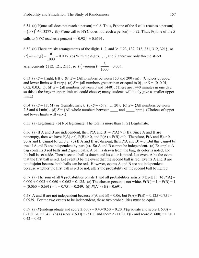
6.60 (a) The choices for Austin and Sara are shown in the table below. The sum of Austin’s picks is in parentheses. Each of the 25 outcomes for Austin could appear with one of the 10 possible choices for Sara, so a tree diagram would have 250 branches.

Austin Sara Number of pairs for Austin with a sum greater than Sara’s pick

Number of pairs for Austin with a sum less than Sara’s pick

1, 1 (2) 1 25 0 1, 2 (3) 2 24 0 1, 3 (4) 3 22 1 1, 4 (5) 4 19 3 1, 5 (6) 5 15 6 2, 1 (3) 6 10 10 2, 2 (4) 7 6 15 2, 3 (5) 8 3 19 2, 4 (6) 9 1 22 2, 5 (7) 10 0 24 3, 1 (4) 3, 2 (5) 3, 3 (6) 3, 4 (7) 3, 5 (8) 4, 1 (5) 4, 2 (6) 4, 3 (7) 4, 4 (8) 4, 5 (9) 5, 1 (6) 5, 2 (7) 5, 3 (8) 5, 4 (9) 5, 5 (10)

(b) The sample space contains 25×10 = 250 outcomes. (c) Count the number of pairs for Austin with a sum greater than each possible value Sara could pick. See the table above. (d) P(Austin wins) = 125/250 = 0.5 (e) Count the number of pairs for Austin with a sum less than each possible value Sara could pick. See the table above. (f) P(Sara wins) = 100/250 = 0.4. (g) The probability of a tie is 25/250 = 0.1. Yes, 0.5 + 0.4 + 0.1 = 1. 6.61 (a) P(under 65) = 0.321 + 0.124 = 0.445. P(65 or older) = 1 − 0.445 = 0.555 OR 0.365 + 0.190 = 0.555. (b) P(tests done) = 0.321 + 0.365 = 0.686. P(tests not done) = 1 − 0.686 = 0.314 OR 0.124 + 0.190 = 0.314. (c) P(A and B) = 0.365; P(A)×P(B) = (0.555)×(0.686) = 0.3807. Thus, events A and B are not independent; tests were done less frequently on older patients than would be the case if these events were independent.

158 Chapter 6

6.62 (a) 1/38. (b) Since 18 slots are red, the probability of winning is 18( ) 0.473738

P red = . (c)

There are 12 winning slots, so P(win a column bet) 12 0.315838

= .

6.63 You should pick the first sequence. Look at the first five rolls in each sequence. All have one G and four R’s, so those probabilities are the same. In the first sequence, you win regardless of the sixth roll; for the second sequence, you win if the sixth roll is G, and for the third

sequence, you win if it is R. The respective probabilities are 42 4 0.0082

6 6⎛ ⎞ ⎛ ⎞×⎜ ⎟ ⎜ ⎟⎝ ⎠ ⎝ ⎠

,

4 22 4 0.00556 6

⎛ ⎞ ⎛ ⎞×⎜ ⎟ ⎜ ⎟⎝ ⎠ ⎝ ⎠

, and 52 4 0.0027

6 6⎛ ⎞ ⎛ ⎞×⎜ ⎟ ⎜ ⎟⎝ ⎠ ⎝ ⎠

.

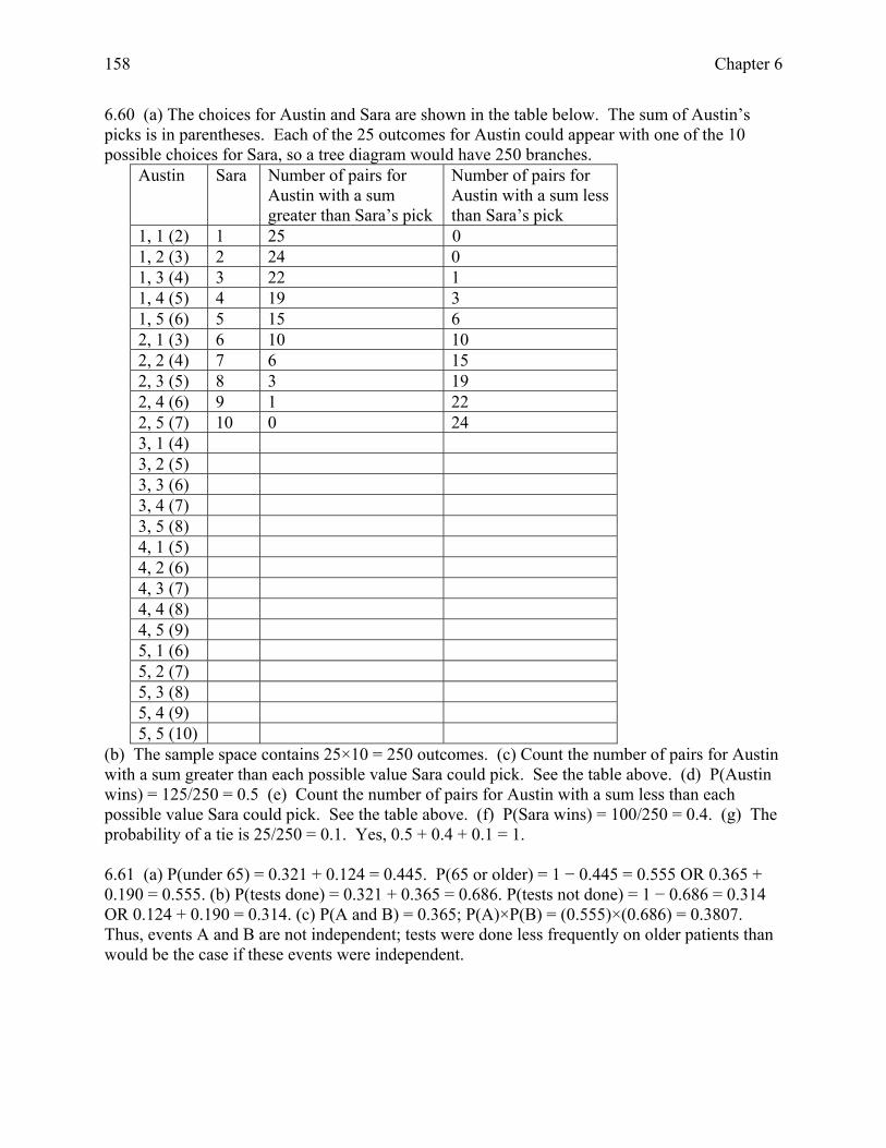
6.64 P(first child is albino) = 0.5×0.5 = 0.25. P(both of two children are albino) = 0.25×0.25 = 0.0625 P(neither is albino) = (1−0.25)×(1−0.25) = 0.5625. 6.65 (a) A Venn diagram is shown below.

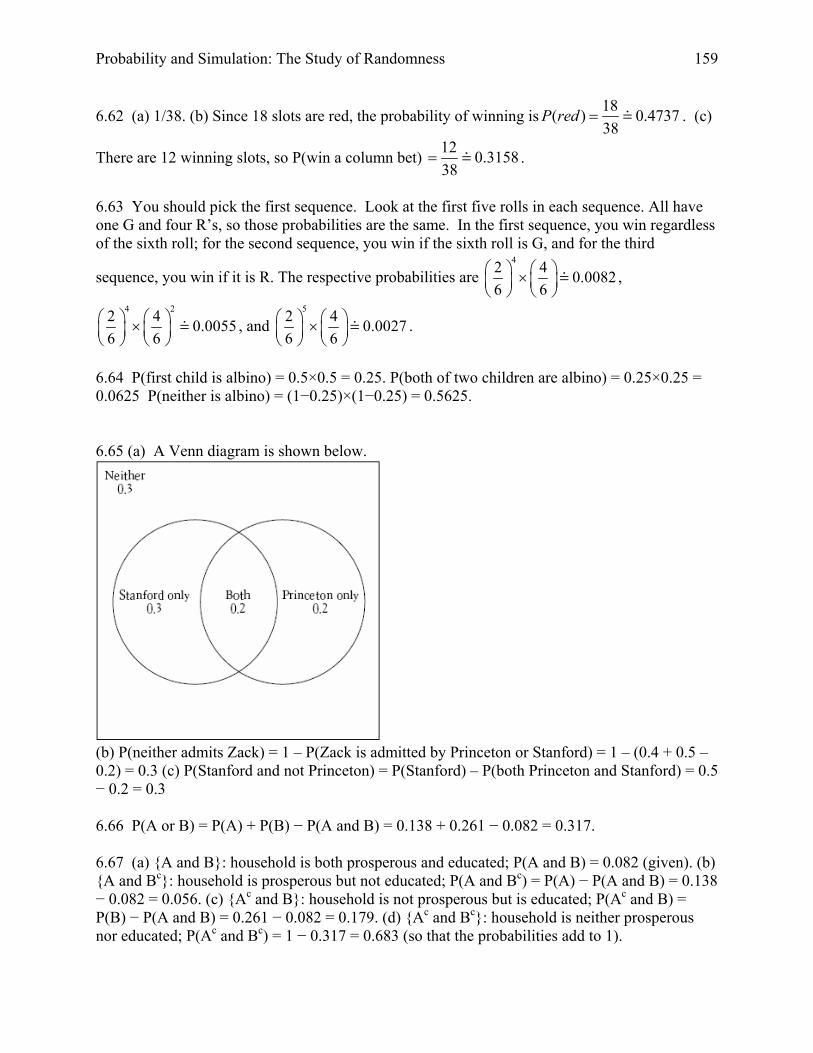
(b) P(neither admits Zack) = 1 – P(Zack is admitted by Princeton or Stanford) = 1 – (0.4 + 0.5 – 0.2) = 0.3 (c) P(Stanford and not Princeton) = P(Stanford) – P(both Princeton and Stanford) = 0.5 − 0.2 = 0.3 6.66 P(A or B) = P(A) + P(B) − P(A and B) = 0.138 + 0.261 − 0.082 = 0.317. 6.67 (a) {A and B}: household is both prosperous and educated; P(A and B) = 0.082 (given). (b) {A and Bc}: household is prosperous but not educated; P(A and Bc) = P(A) − P(A and B) = 0.138 − 0.082 = 0.056. (c) {Ac and B}: household is not prosperous but is educated; P(Ac and B) = P(B) − P(A and B) = 0.261 − 0.082 = 0.179. (d) {Ac and Bc}: household is neither prosperous nor educated; P(Ac and Bc) = 1 − 0.317 = 0.683 (so that the probabilities add to 1).


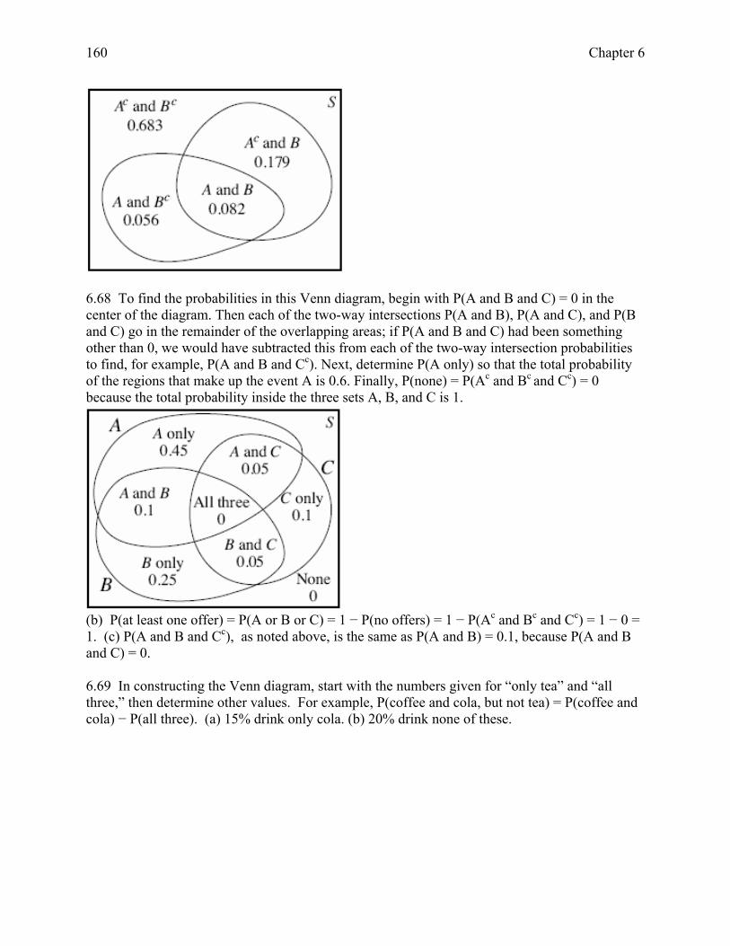
6.68 To find the probabilities in this Venn diagram, begin with P(A and B and C) = 0 in the center of the diagram. Then each of the two-way intersections P(A and B), P(A and C), and P(B and C) go in the remainder of the overlapping areas; if P(A and B and C) had been something other than 0, we would have subtracted this from each of the two-way intersection probabilities to find, for example, P(A and B and Cc). Next, determine P(A only) so that the total probability of the regions that make up the event A is 0.6. Finally, P(none) = P(Ac and Bc and Cc) = 0 because the total probability inside the three sets A, B, and C is 1.

(b) P(at least one offer) = P(A or B or C) = 1 − P(no offers) = 1 − P(Ac and Bc and Cc) = 1 − 0 = 1. (c) P(A and B and Cc), as noted above, is the same as P(A and B) = 0.1, because P(A and B and C) = 0. 6.69 In constructing the Venn diagram, start with the numbers given for “only tea” and “all three,” then determine other values. For example, P(coffee and cola, but not tea) = P(coffee and cola) − P(all three). (a) 15% drink only cola. (b) 20% drink none of these.

160 Chapter 6

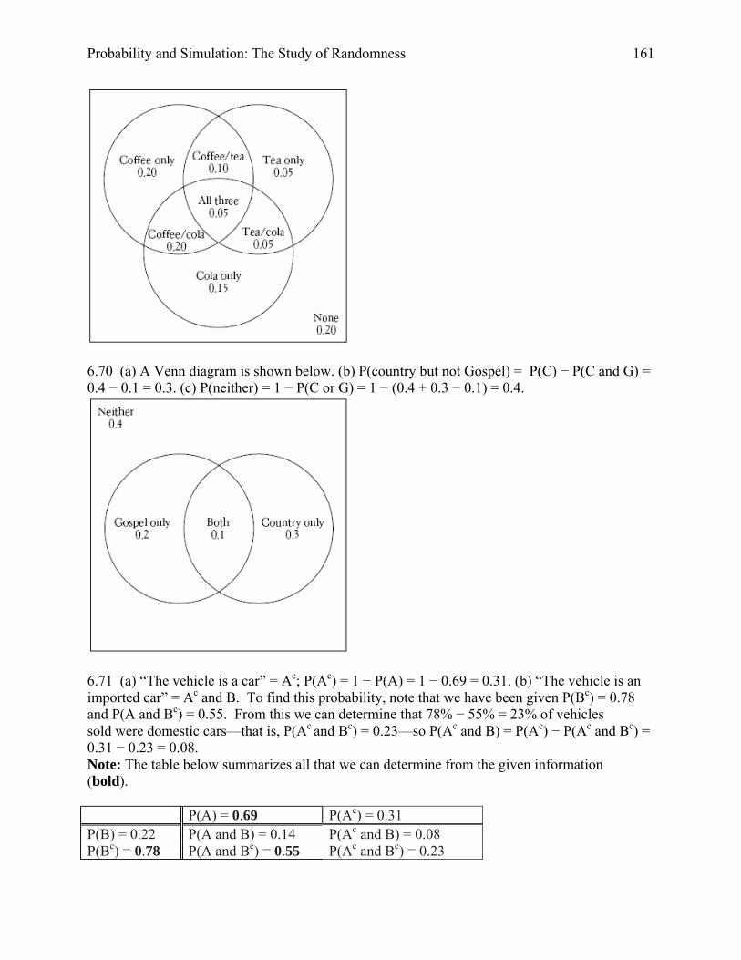
6.70 (a) A Venn diagram is shown below. (b) P(country but not Gospel) = P(C) − P(C and G) = 0.4 − 0.1 = 0.3. (c) P(neither) = 1 − P(C or G) = 1 − (0.4 + 0.3 − 0.1) = 0.4.

6.71 (a) “The vehicle is a car” = Ac; P(Ac) = 1 − P(A) = 1 − 0.69 = 0.31. (b) “The vehicle is an imported car” = Ac and B. To find this probability, note that we have been given P(Bc) = 0.78 and P(A and Bc) = 0.55. From this we can determine that 78% − 55% = 23% of vehicles sold were domestic cars—that is, P(Ac and Bc) = 0.23—so P(Ac and B) = P(Ac) − P(Ac and Bc) = 0.31 − 0.23 = 0.08. Note: The table below summarizes all that we can determine from the given information (bold). P(A) = 0.69 P(Ac) = 0.31 P(B) = 0.22 P(A and B) = 0.14 P(Ac and B) = 0.08 P(Bc) = 0.78 P(A and Bc) = 0.55 P(Ac and Bc) = 0.23


P(The vehicle is an imported car) = P(Ac and B) = P(B) – P(A and B) = 0.22 − 0.14 = 0.08.

(c) ( ) ( )( )

0.08| 0.36360.22

cc

P A andBP A B

P B= = (d) The events Ac and B are not independent, if

they were, ( | )cP A B would be the same as ( )cP A . 6.72 Although this exercise does not call for a tree diagram, one is shown below. The numbers on the right side of the tree are found by the multiplication rule; for example, P(“regular” and “≥ $20”) = P(R and T) = P(R) × P(T | R) = (0.4)×(0.3) = 0.12. The probability that the next customer pays at least $20 is P(T ) = 0.12 + 0.175 + 0.15 = 0.445.

Customer

Yes 0.12

Premium

Regular

≥$20Grade

Midrange

No 0.10

Yes 0.15

No 0.175

Yes 0.175

No 0.280.4

0.4

0.6

0.5

0.50.7

0.25

0.3

0.35

6.73 ( $20) 0.15( | $20) 0.337

($20) 0.445P Premium

P PremiumP

∩= = = . About 34%.

6.74 P(A and B) = P(A) P(B | A) = (0.46)(0.32) = 0.1472. 6.75 Let F = {dollar falls} and R = {renegotiation demanded}, then P(F and R) = P(F)×P(R|F) = (0.4)×(0.8) = 0.32. 6.76 (a) & (b) These probabilities are:

P(1st card ♠) = 13 0.2552

=

162 Chapter 6

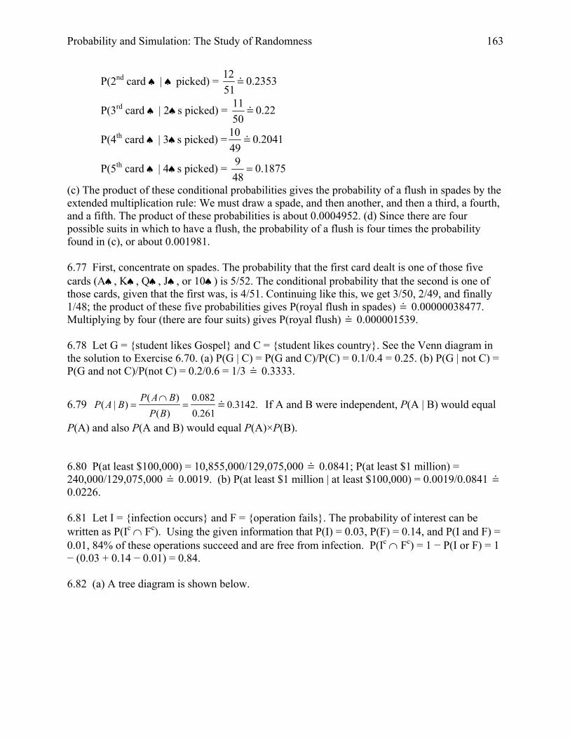
P(2nd card ♠ | ♠ picked) = 12 0.235351

P(3rd card ♠ | 2♠s picked) = 11 0.2250

P(4th card ♠ | 3♠s picked) = 10 0.204149

P(5th card ♠ | 4♠s picked) = 9 0.187548

=

(c) The product of these conditional probabilities gives the probability of a flush in spades by the extended multiplication rule: We must draw a spade, and then another, and then a third, a fourth, and a fifth. The product of these probabilities is about 0.0004952. (d) Since there are four possible suits in which to have a flush, the probability of a flush is four times the probability found in (c), or about 0.001981. 6.77 First, concentrate on spades. The probability that the first card dealt is one of those five cards (A♠, K♠, Q♠, J♠, or 10♠) is 5/52. The conditional probability that the second is one of those cards, given that the first was, is 4/51. Continuing like this, we get 3/50, 2/49, and finally 1/48; the product of these five probabilities gives P(royal flush in spades) 0.00000038477. Multiplying by four (there are four suits) gives P(royal flush) 0.000001539. 6.78 Let G = {student likes Gospel} and C = {student likes country}. See the Venn diagram in the solution to Exercise 6.70. (a) P(G | C) = P(G and C)/P(C) = 0.1/0.4 = 0.25. (b) P(G | not C) = P(G and not C)/P(not C) = 0.2/0.6 = 1/3 0.3333.

6.79 ( ) 0.082( | ) 0.3142.

( ) 0.261P A B

P A BP B∩

= = If A and B were independent, P(A | B) would equal

P(A) and also P(A and B) would equal P(A)×P(B). 6.80 P(at least $100,000) = 10,855,000/129,075,000 0.0841; P(at least $1 million) = 240,000/129,075,000 0.0019. (b) P(at least $1 million | at least $100,000) = 0.0019/0.0841 0.0226. 6.81 Let I = {infection occurs} and F = {operation fails}. The probability of interest can be written as P(Ic ∩ Fc). Using the given information that P(I) = 0.03, P(F) = 0.14, and P(I and F) = 0.01, 84% of these operations succeed and are free from infection. P(Ic ∩ Fc) = 1 − P(I or F) = 1 − (0.03 + 0.14 − 0.01) = 0.84. 6.82 (a) A tree diagram is shown below.


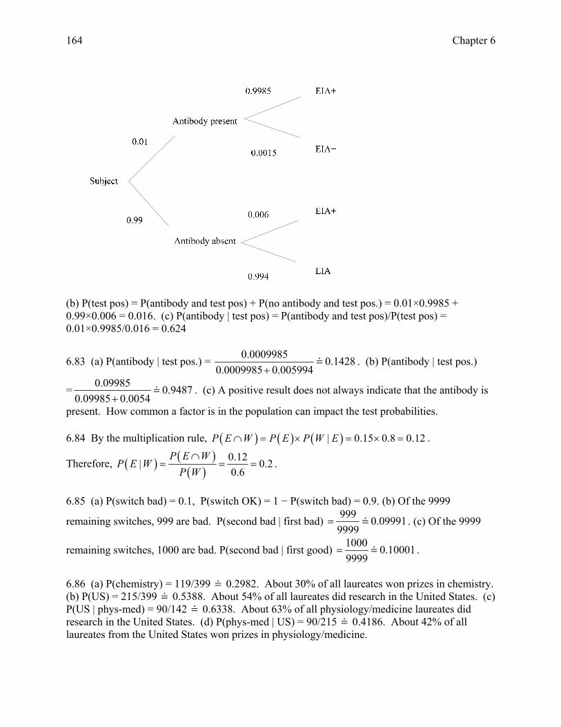
(b) P(test pos) = P(antibody and test pos) + P(no antibody and test pos.) = 0.01×0.9985 + 0.99×0.006 = 0.016. (c) P(antibody | test pos) = P(antibody and test pos)/P(test pos) = 0.01×0.9985/0.016 = 0.624

6.83 (a) P(antibody | test pos.) = 0.0009985 0.14280.0009985 0.005994+

. (b) P(antibody | test pos.)

= 0.09985 0.94870.09985 0.0054+

. (c) A positive result does not always indicate that the antibody is

present. How common a factor is in the population can impact the test probabilities. 6.84 By the multiplication rule, ( ) ( ) ( )| 0.15 0.8 0.12P E W P E P W E∩ = × = × = .

Therefore, ( ) ( )( )

0.12| 00.6

P E WP E W

P W∩

= = .2= .

6.85 (a) P(switch bad) = 0.1, P(switch OK) = 1 − P(switch bad) = 0.9. (b) Of the 9999

remaining switches, 999 are bad. P(second bad | first bad) 999 0.099919999

= . (c) Of the 9999

remaining switches, 1000 are bad. P(second bad | first good) 1000 0.100019999

= .

6.86 (a) P(chemistry) = 119/399 0.2982. About 30% of all laureates won prizes in chemistry. (b) P(US) = 215/399 0.5388. About 54% of all laureates did research in the United States. (c) P(US | phys-med) = 90/142 0.6338. About 63% of all physiology/medicine laureates did research in the United States. (d) P(phys-med | US) = 90/215 0.4186. About 42% of all laureates from the United States won prizes in physiology/medicine.

164 Chapter 6

6.87 Let W be the event “the person is a woman” and P be “the person earned a professional degree.” (a) P(W) = 1119/1944 0.5756. (b) P(W | P) = 39/83 0.4699. (c) W and P are not independent; if they were, the two probabilities in (a) and (b), P(W) and P(W | P), would be equal. 6.88 (a) P(Jack) = 1/13. (b) P(5 on second | Jack on first) = 1/12. (c) P(Jack on first and 5 on second) = P(jack on first) × P(5 on second | Jack on first) = (1/13) × (1/12) = 1/156. (d) P(both cards greater than 5) = P(first card greater than 5) × P(second card greater than 5 | first card greater than 5) = (8/13) × (7/12) = 56/156 0.359. 6.89 Let M be the event “the person is a man” and B be “the person earned a bachelor’s degree.” (a) P(M) = 825/1944 0.4244 (b) P(B|M) = 559/825 0.6776 (c) P(M ∩ B) = P(M)⋅ P(B | M) = (0.4244)×(0.6776) 0.2876. This agrees with the directly computed probability: P(M and B) = 559/1944 0.2876. 6.90 (a) P(C) = 0.20, P(A) = 0.10, P(A | C) = 0.05. (b) P(A and C) = P(C) × P(A | C) = (0.20)×(0.05) = 0.01.

6.91 ( ) 0.01( | ) 0.10

( ) 0.10P C A

P C AP A∩

= = = , so 10% of A students are involved in an accident.

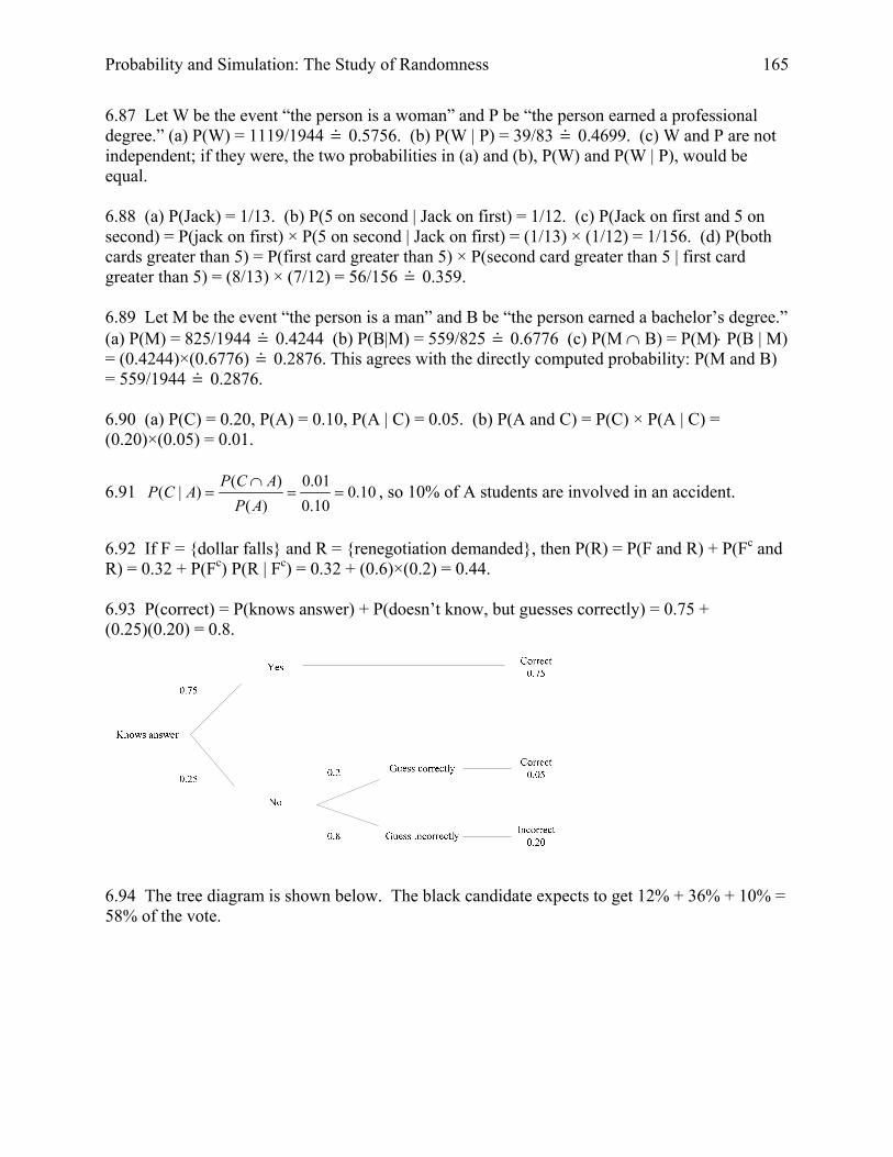
6.92 If F = {dollar falls} and R = {renegotiation demanded}, then P(R) = P(F and R) + P(Fc and R) = 0.32 + P(Fc) P(R | Fc) = 0.32 + (0.6)×(0.2) = 0.44. 6.93 P(correct) = P(knows answer) + P(doesn’t know, but guesses correctly) = 0.75 + (0.25)(0.20) = 0.8.

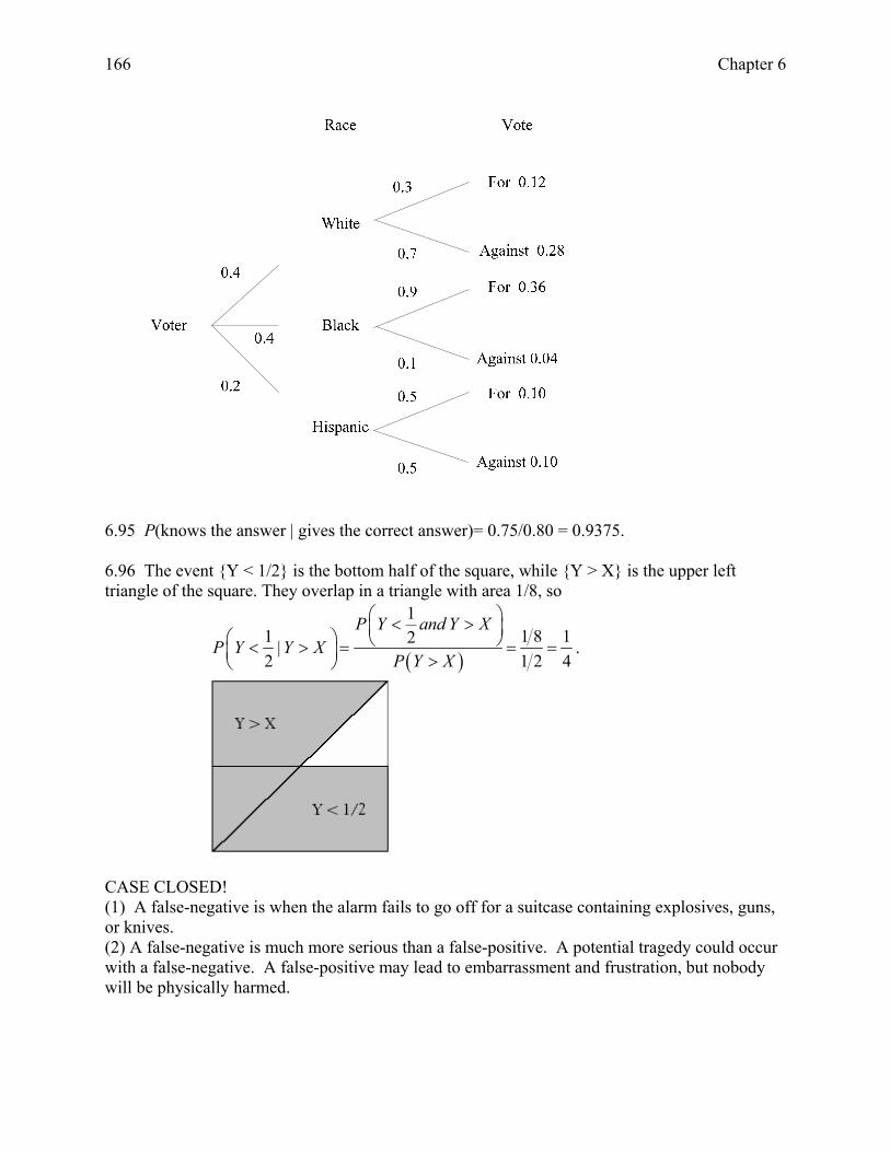
6.94 The tree diagram is shown below. The black candidate expects to get 12% + 36% + 10% = 58% of the vote.


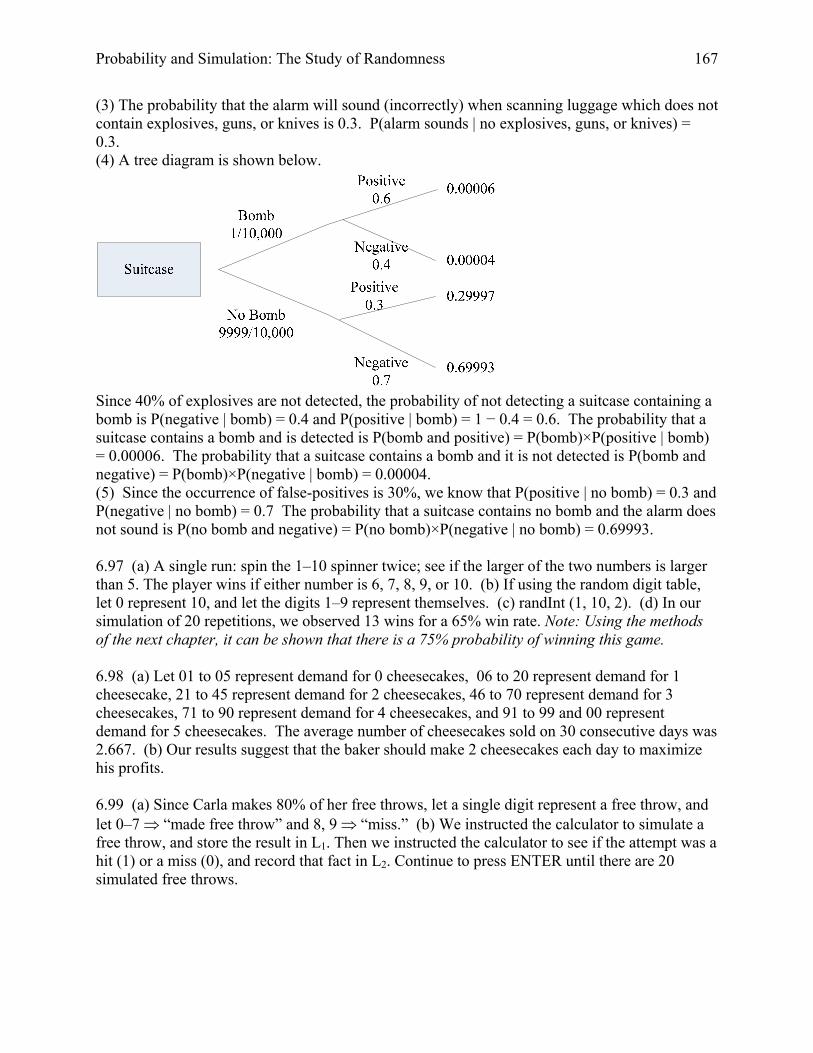
6.95 P(knows the answer | gives the correct answer)= 0.75/0.80 = 0.9375. 6.96 The event {Y < 1/2} is the bottom half of the square, while {Y > X} is the upper left triangle of the square. They overlap in a triangle with area 1/8, so

( )

11 12|2 1

P Y and Y XP Y Y X

P Y X

⎛ ⎞< >⎜ ⎟⎛ ⎞ ⎝ ⎠< > = = =⎜ ⎟ >⎝ ⎠8 12 4

.

CASE CLOSED! (1) A false-negative is when the alarm fails to go off for a suitcase containing explosives, guns, or knives. (2) A false-negative is much more serious than a false-positive. A potential tragedy could occur with a false-negative. A false-positive may lead to embarrassment and frustration, but nobody will be physically harmed.

166 Chapter 6

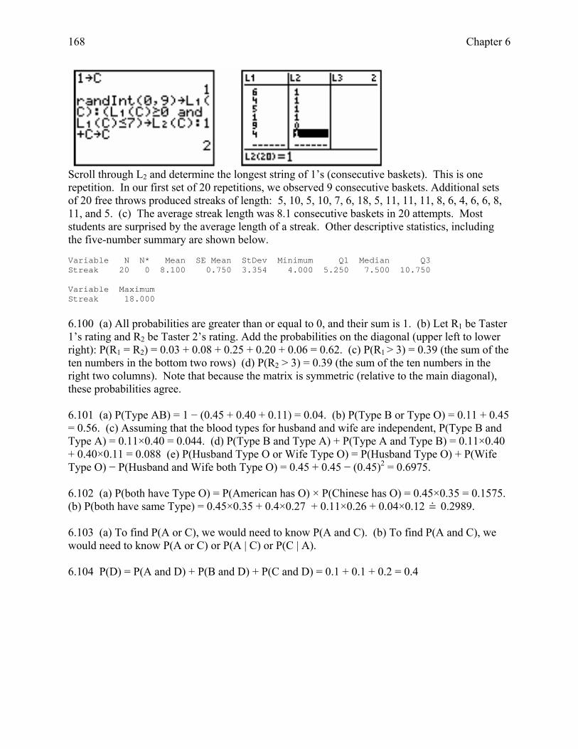
(3) The probability that the alarm will sound (incorrectly) when scanning luggage which does not contain explosives, guns, or knives is 0.3. P(alarm sounds | no explosives, guns, or knives) = 0.3. (4) A tree diagram is shown below.

Since 40% of explosives are not detected, the probability of not detecting a suitcase containing a bomb is P(negative | bomb) = 0.4 and P(positive | bomb) = 1 − 0.4 = 0.6. The probability that a suitcase contains a bomb and is detected is P(bomb and positive) = P(bomb)×P(positive | bomb) = 0.00006. The probability that a suitcase contains a bomb and it is not detected is P(bomb and negative) = P(bomb)×P(negative | bomb) = 0.00004. (5) Since the occurrence of false-positives is 30%, we know that P(positive | no bomb) = 0.3 and P(negative | no bomb) = 0.7 The probability that a suitcase contains no bomb and the alarm does not sound is P(no bomb and negative) = P(no bomb)×P(negative | no bomb) = 0.69993. 6.97 (a) A single run: spin the 1–10 spinner twice; see if the larger of the two numbers is larger than 5. The player wins if either number is 6, 7, 8, 9, or 10. (b) If using the random digit table, let 0 represent 10, and let the digits 1–9 represent themselves. (c) randInt (1, 10, 2). (d) In our simulation of 20 repetitions, we observed 13 wins for a 65% win rate. Note: Using the methods of the next chapter, it can be shown that there is a 75% probability of winning this game. 6.98 (a) Let 01 to 05 represent demand for 0 cheesecakes, 06 to 20 represent demand for 1 cheesecake, 21 to 45 represent demand for 2 cheesecakes, 46 to 70 represent demand for 3 cheesecakes, 71 to 90 represent demand for 4 cheesecakes, and 91 to 99 and 00 represent demand for 5 cheesecakes. The average number of cheesecakes sold on 30 consecutive days was 2.667. (b) Our results suggest that the baker should make 2 cheesecakes each day to maximize his profits. 6.99 (a) Since Carla makes 80% of her free throws, let a single digit represent a free throw, and let 0–7 ⇒ “made free throw” and 8, 9 ⇒ “miss.” (b) We instructed the calculator to simulate a free throw, and store the result in L1. Then we instructed the calculator to see if the attempt was a hit (1) or a miss (0), and record that fact in L2. Continue to press ENTER until there are 20 simulated free throws.


Scroll through L2 and determine the longest string of 1’s (consecutive baskets). This is one repetition. In our first set of 20 repetitions, we observed 9 consecutive baskets. Additional sets of 20 free throws produced streaks of length: 5, 10, 5, 10, 7, 6, 18, 5, 11, 11, 11, 8, 6, 4, 6, 6, 8, 11, and 5. (c) The average streak length was 8.1 consecutive baskets in 20 attempts. Most students are surprised by the average length of a streak. Other descriptive statistics, including the five-number summary are shown below. Variable N N* Mean SE Mean StDev Minimum Q1 Median Q3 Streak 20 0 8.100 0.750 3.354 4.000 5.250 7.500 10.750 Variable Maximum Streak 18.000

6.100 (a) All probabilities are greater than or equal to 0, and their sum is 1. (b) Let R1 be Taster 1’s rating and R2 be Taster 2’s rating. Add the probabilities on the diagonal (upper left to lower right): P(R1 = R2) = 0.03 + 0.08 + 0.25 + 0.20 + 0.06 = 0.62. (c) P(R1 > 3) = 0.39 (the sum of the ten numbers in the bottom two rows) (d) P(R2 > 3) = 0.39 (the sum of the ten numbers in the right two columns). Note that because the matrix is symmetric (relative to the main diagonal), these probabilities agree. 6.101 (a) P(Type AB) = 1 − (0.45 + 0.40 + 0.11) = 0.04. (b) P(Type B or Type O) = 0.11 + 0.45 = 0.56. (c) Assuming that the blood types for husband and wife are independent, P(Type B and Type A) = 0.11×0.40 = 0.044. (d) P(Type B and Type A) + P(Type A and Type B) = 0.11×0.40 + 0.40×0.11 = 0.088 (e) P(Husband Type O or Wife Type O) = P(Husband Type O) + P(Wife Type O) − P(Husband and Wife both Type O) = 0.45 + 0.45 − (0.45)2 = 0.6975. 6.102 (a) P(both have Type O) = P(American has O) × P(Chinese has O) = 0.45×0.35 = 0.1575. (b) P(both have same Type) = 0.45×0.35 + 0.4×0.27 + 0.11×0.26 + 0.04×0.12 0.2989. 6.103 (a) To find P(A or C), we would need to know P(A and C). (b) To find P(A and C), we would need to know P(A or C) or P(A | C) or P(C | A). 6.104 P(D) = P(A and D) + P(B and D) + P(C and D) = 0.1 + 0.1 + 0.2 = 0.4

168 Chapter 6

6.105 Let H = {adult belongs to health club} and G = {adult goes to club at least twice a week}. P(G and H) = P(H) × P(G | H) = (0.1) × (0.4) = 0.04. 6.106 P(B | A) = P(both tosses have the same outcome | head on first toss) = P(both heads)/P(head on first toss) = 0.25/0.5 = 0.5. P(B) = P(both tosses have same outcome) = 2/4 = 0.5. Since P(B | A) = P(B), events A and B are independent. 6.107 Let R1 be Taster 1’s rating and R2 be Taster 2’s rating. P(R1 = 3) = 0.01 + 0.05 + 0.25 + 0.05 + 0.01 = 0.37 and P(R2 > 3 ∩ R1 = 3) = 0.05 + 0.01 = 0.06, so

2 12 1

1

( 3 3)( 3 | 3)

( 3)0.06 .16220.37

P R RP R R

P R> ∩ =

> = ==

=

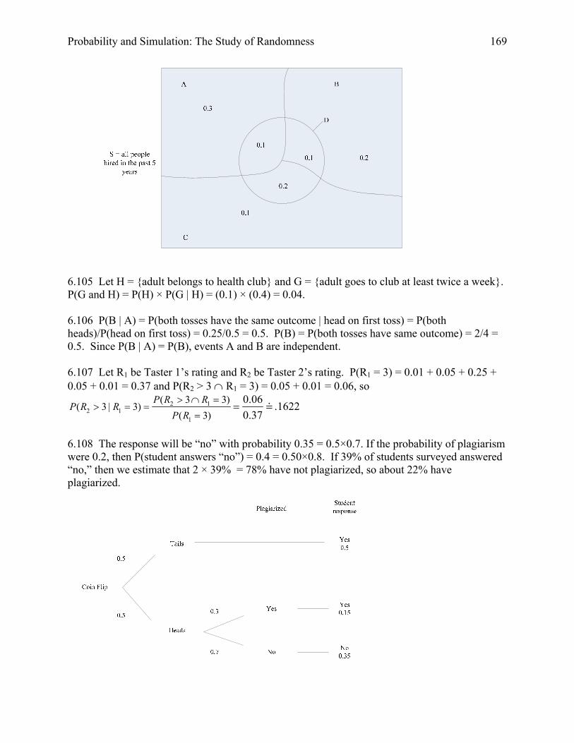
6.108 The response will be “no” with probability 0.35 = 0.5×0.7. If the probability of plagiarism were 0.2, then P(student answers “no”) = 0.4 = 0.50×0.8. If 39% of students surveyed answered “no,” then we estimate that 2 × 39% = 78% have not plagiarized, so about 22% have plagiarized.


Documents

148 Chapter 6 Chapter 6 - westada.org