1/33

Nonrigid Registration

2/33

Transformations are more complex

Rigid has only 6 DOF—three shifts and three angles

Important non-rigid transformations

• Similarity: 7 DOF

• Affine: 12 DOF

• Curved: Typically DOF = 100 to 1000.

3/33

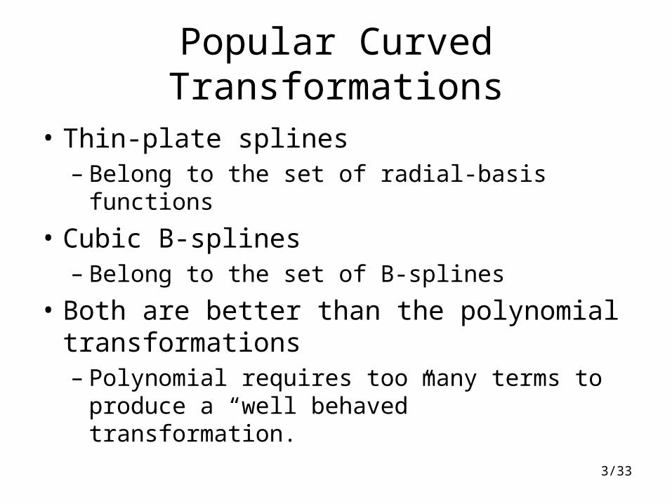
Popular Curved Transformations

• Thin-plate splines– Belong to the set of radial-basis functions

• Cubic B-splines– Belong to the set of B-splines

• Both are better than the polynomial transformations– Polynomial requires too many terms to

produce a “well behaved” transformation.

4/33

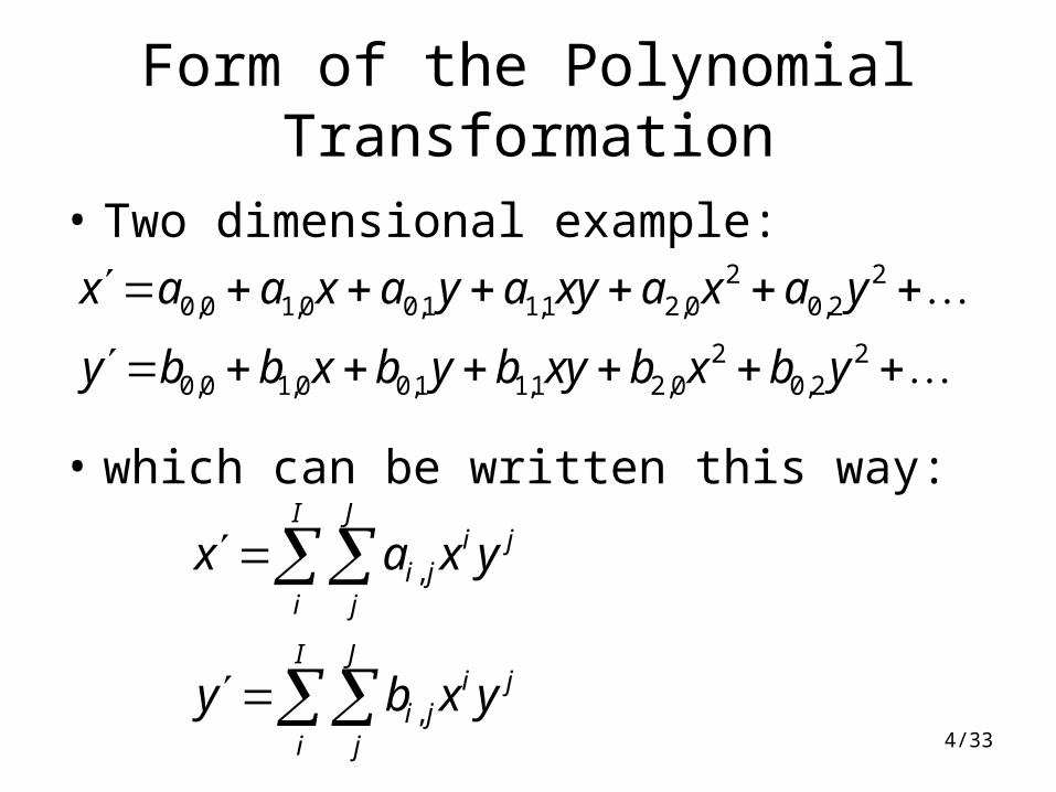
Form of the Polynomial Transformation

• Two dimensional example:2 2

0,0 1,0 0,1 1,1 2,0 0,2

2 20,0 1,0 0,1 1,1 2,0 0,2

x a a x a y a xy a x a y

y b b x b y b xy b x b y

,

,

I Ji j

i ji j

I Ji j

i ji j

x a x y

y b x y

• which can be written this way:

5/33

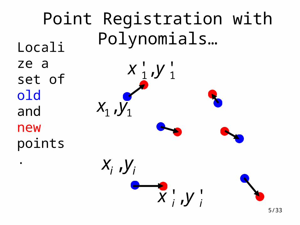
Point Registration with Polynomials…

Localize a set of old and new points.

' , 'i ix y

1 1,x y

,i ix y

1 1' , 'x y

6/33

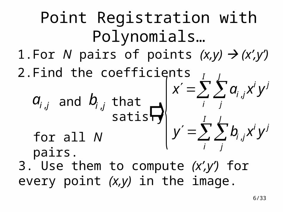
Point Registration with Polynomials…

1. For N pairs of points (x,y) (x’,y’)

2. Find the coefficients

,i ja and ,i jb that satisfy

,

,

I Ji j

i ji j

I Ji j

i ji j

x a x y

y b x y

3. Use them to compute (x’,y’) for every point (x,y) in the image.

for all N pairs.

7/33

Method for Finding Coefficients

• Requires solution of Ax = b– A depends on the initial points– b depends on final points– x contains the coefficients

• See handout – Polynomial Transformation.doc

8/33

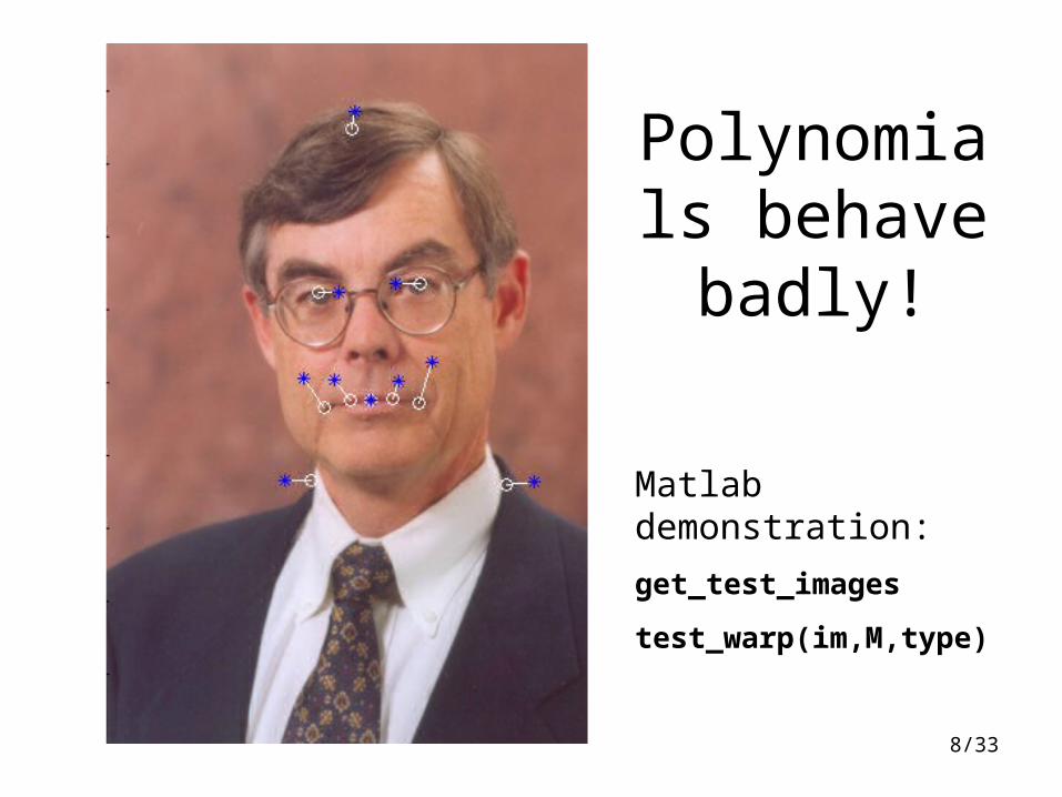
Matlab demonstration:

get_test_images

test_warp(im,M,type)

Polynomials behave badly!

9/33

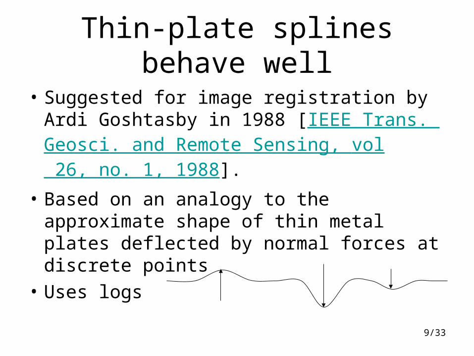
Thin-plate splines behave well

• Suggested for image registration by Ardi Goshtasby in 1988 [IEEE Trans. Geosci. and Remote Sensing, vol 26, no. 1, 1988].

• Based on an analogy to the approximate shape of thin metal plates deflected by normal forces at discrete points

• Uses logs

10/33

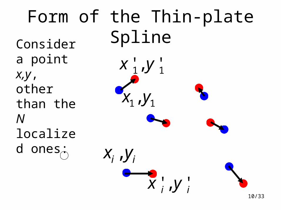
Consider a point x,y, other than the N localized ones:

' , 'i ix y

1 1,x y

,i ix y

1 1' , 'x y

Form of the Thin-plate Spline

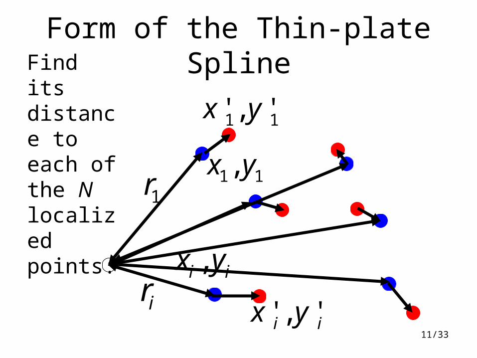
11/33

Find its distance to each of the N localized points:

' , 'i ix y

1 1,x y

,i ix y

1 1' , 'x y

Form of the Thin-plate Spline

ir

1r

12/33

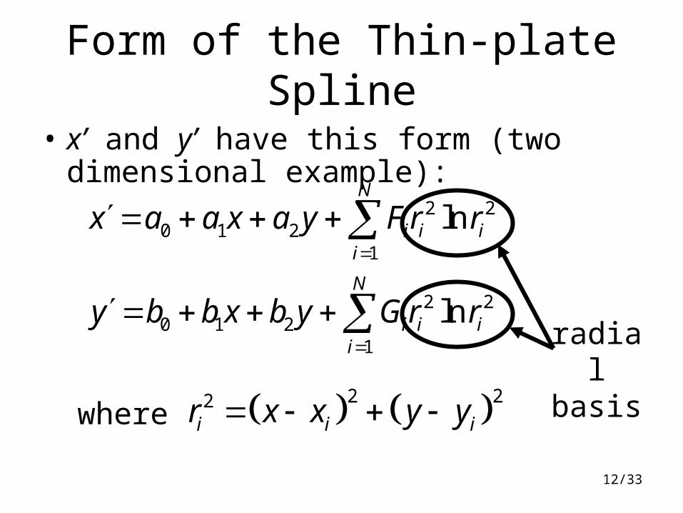
Form of the Thin-plate Spline

• x’ and y’ have this form (two dimensional example):

2 20 1 2

1

2 20 1 2

1

ln

ln

N

i i ii

N

i i ii

x a a x a y F r r

y b b x b y G r r

2 22i i ir x x y y where

radial basis

13/33

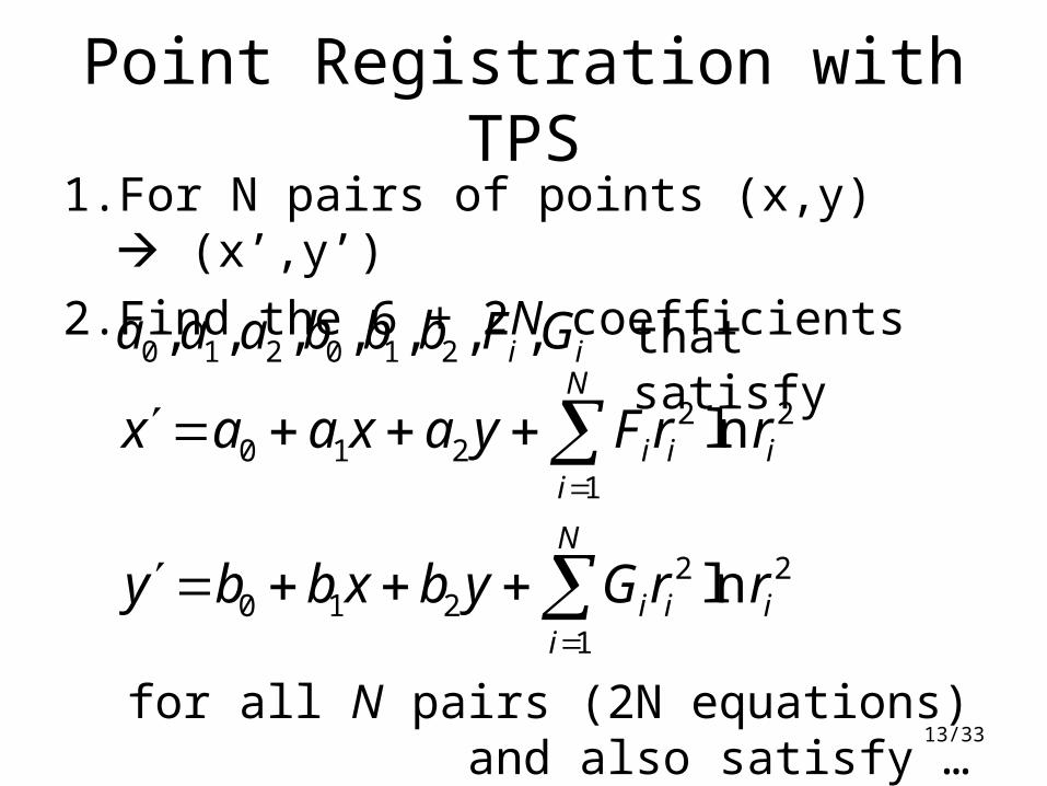
Point Registration with TPS1. For N pairs of points (x,y) (x’,y’)

2. Find the 6 + 2N coefficients

2 20 1 2

1

2 20 1 2

1

ln

ln

N

i i ii

N

i i ii

x a a x a y F r r

y b b x b y G r r

that satisfy0 1 2 0 1 2, , , , , , ,i ia a a b b b F G

for all N pairs (2N equations) and also satisfy …

14/33

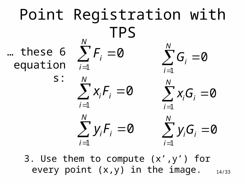
… these 6 equations:

Point Registration with TPS

3. Use them to compute (x’,y’) for every point (x,y) in the image.

1

1

1

0

0

0

N

ii

N

i ii

N

i ii

F

x F

y F

1

1

1

0

0

0

N

ii

N

i ii

N

i ii

G

x G

y G

15/33

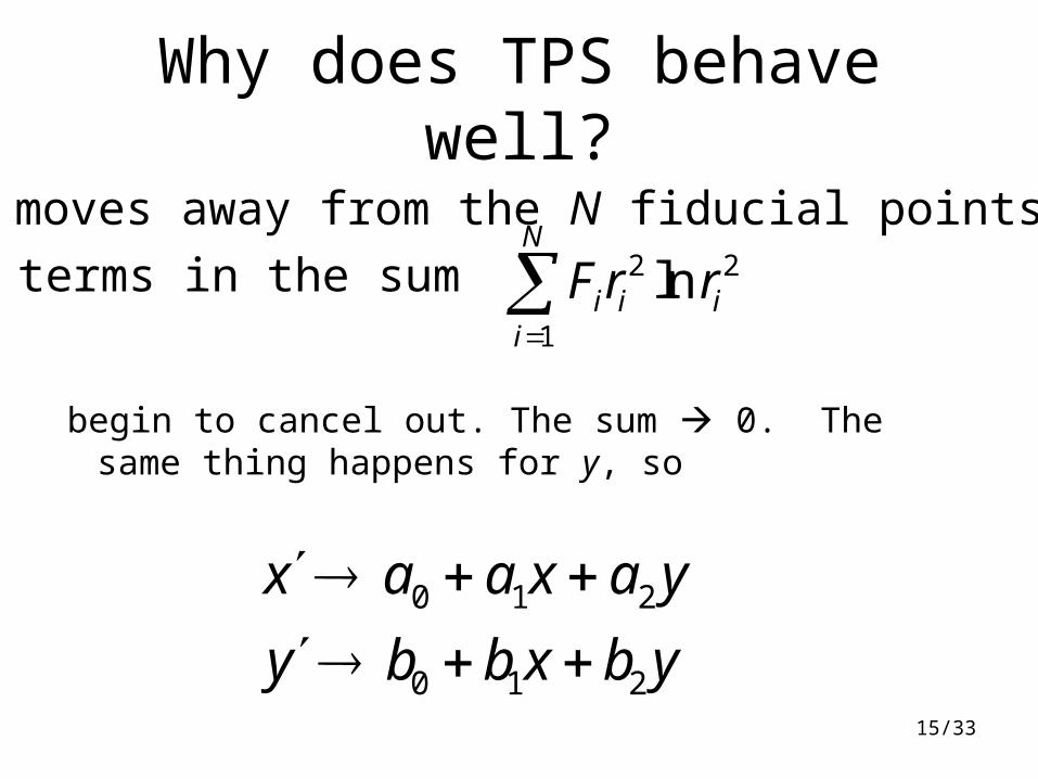
Why does TPS behave well?

2 2

1

lnN

i i ii

F r r

begin to cancel out. The sum 0. The same thing happens for y, so

0 1 2

0 1 2

x a a x a y

y b b x b y

As x moves away from the N fiducial points,

the terms in the sum

16/33

Method for Finding Coefficients

• Requires solution of Ax = b– A depends on the initial points– b depends on final points– x contains the coefficients

• See handout – Thin-Plate Spline Transformation.doc

• Example of use in medical image registration: Meyer, Med. Im. Analy, vol 1, no. 3, pp. 195-206 (1996/7)

(same as for polynomials)

17/33

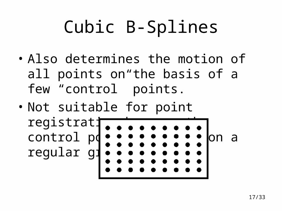
Cubic B-Splines

• Also determines the motion of all points on the basis of a few “control” points.

• Not suitable for point registration because the control points must lie on a regular grid.

18/33

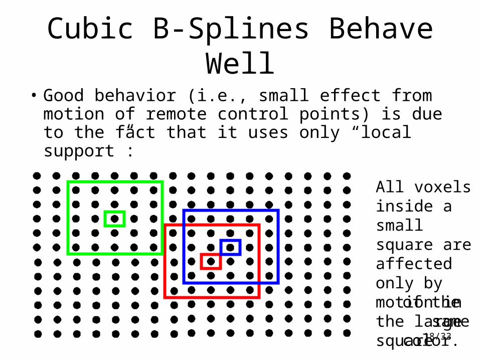
Cubic B-Splines Behave Well

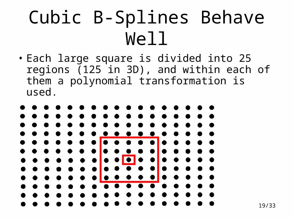
• Good behavior (i.e., small effect from motion of remote control points) is due to the fact that it uses only “local support”:

All voxels inside a small square are affected only by motion in the large squareof the same color.

19/33

Cubic B-Splines Behave Well

• Each large square is divided into 25 regions (125 in 3D), and within each of them a polynomial transformation is used.

20/33

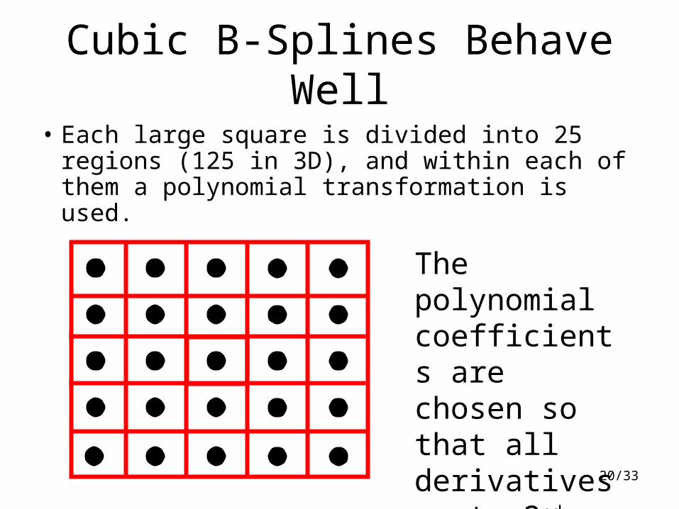
Cubic B-Splines Behave Well

• Each large square is divided into 25 regions (125 in 3D), and within each of them a polynomial transformation is used.

The polynomial coefficients are chosen so that all derivatives up to 2nd order are continuous.

21/33

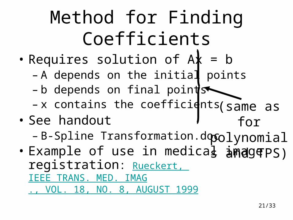
Method for Finding Coefficients

• Requires solution of Ax = b– A depends on the initial points– b depends on final points– x contains the coefficients

• See handout – B-Spline Transformation.doc

• Example of use in medical image registration: Rueckert, IEEE TRANS. MED. IMAG., VOL. 18, NO. 8, AUGUST 1999

(same as for polynomials and TPS)

22/33

Continuous Derivatives

• Continuous derivatives reduce “kinks”.

• Both polynomials and thin-place-splines are continuous in all derivatives.

• Cubic B-splines are continuous in all derivatives except 3rd order. – (All derivatives higher than 3rd order are

zero.)

23/33

Nonrigid Intensity Registration

• Let B’(x,y) = B(x’,y’) be a transformed version of image B(x,y).

• Let D(A,B’) be a measure of the dissimilarity of A and B’

– e.g., SAD, or –I(A,B’)

• Search for the transformation,(x’,y’) = T(x,y), that makes D(A,B’) small.

– Loop: Adjust control points, find coefficients, calculate D(A,B(T(x,y))

24/33

Regularization

• It may be desired to limit the variation of the transformation T in some way.– keep some derivatives small– keep the Jacobian close to 1

• Define a variation function, V(T) that is large when the variation in T large

• Search for T that makes C = D(A,B’) + V(T) small.

25/33

Search Techniques

• Grid, steepest descent, Powell’s method, simplex method [Numerical Recipes]

• Stochastic methods (use randomness)– Simulated annealing– Genetic algorithms

• Course-to-fine search– change discretization of coefficients of T– change discretization of images

26/33

End of nonrigid registration and Beginning of Course Review

27/33

Geometrical Transformations

Rigid transformations– All distances remain constant– x’ = Rx + t

• Nonrigid transformations– Distances change but lines remain straight– Curved transformations

• Polynomial• Thin-plate spline• B-spline

28/33

Registration Dichotomy

• Prospective– Something is done to objects before imaging.– Fiducials may be added to objects and point

registration done.

• Retrospective– Nothing is done to objects before imaging.– Anatomical points (rarely reliable)– Surfaces (rarely reliable)– Intensity

29/33

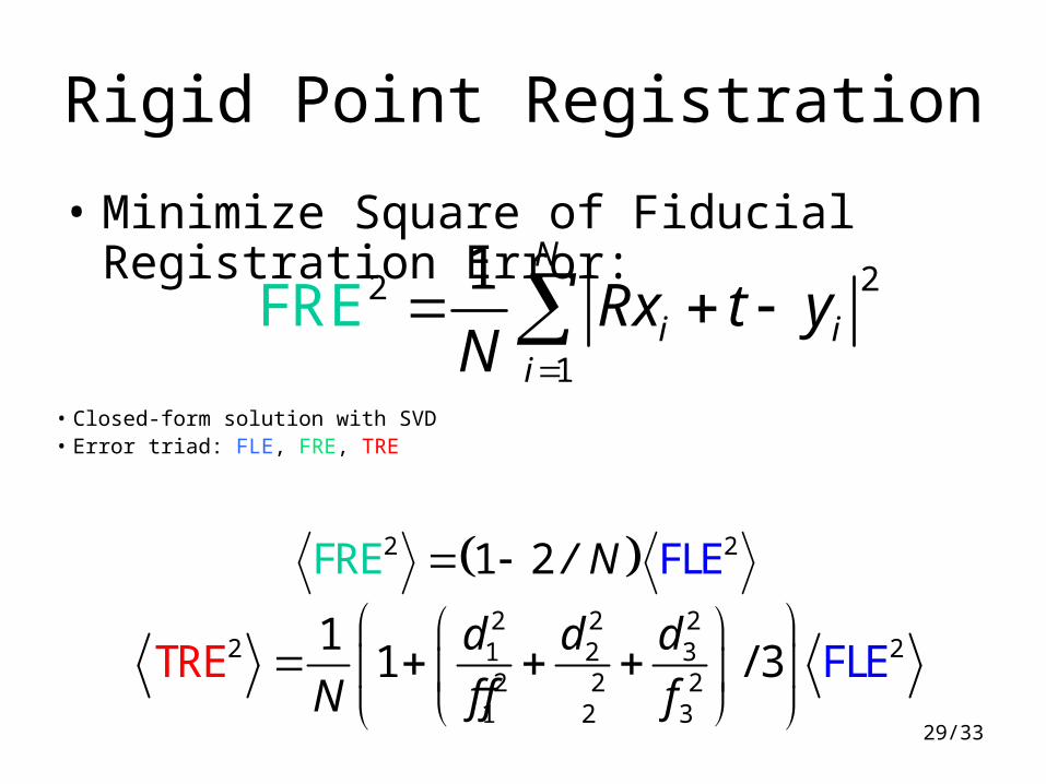
Rigid Point Registration

• Minimize Square of Fiducial Registration Error: 22

1

RE1

FN

i ii

Rx t yN

• Closed-form solution with SVD• Error triad: FLE, FRE, TRE

2 21 2 / N F E FLER2 2 2

2 21 2 32 2 21 2 3

11 / 3

d d d

N f f f

T E FLER

30/33

Intensity Registration

• For intramodality– Sum absolute differences– Sum absolute differences

• If B = aA + c: Correlation coefficient

• For all modalities– Entropy– Mutual Information– Normalized Mutual Information

31/33

All Done!