1.1 The data-handling cycle - Collins Educationresources.collins.co.uk/free/AQAGCSEStatisticsAnswers.pdf · b Students obtain higher marks if they take a maths exam in the ... inter-quartile

1.1 The data-handling cycle

Answers to Exercise 1A

1 These answers are just suggestions and there are many correct alternatives:

a Girls spend longer than boys doing their homework.

b Students obtain higher marks if they take a maths exam in the morning rather than the afternoon.

c More people take skiing holidays now than they did 20 years ago.

d Life expectancy is longer in the south of England than the north.

e Rainfall varies more in Scotland than Wales.

2 For some of these, it may be possible to use either:

a Probably primary, but there may be some secondary data available on the Internet.

b Again, probably primary, but there may be some secondary data available on the Internet.

c Probably secondary, but it may be possible for students to do their own survey if they can get a large enough sample and matched it with another sample taken from the generation that are 20 years older.

d Secondary.

e Secondary.

3 These answers are just suggestions, and there are many correct alternatives:

a Take a random sample (possibly stratified by years) of 50 boys and 50 girls from a school and ask them how long they spent on their homework last night.

b Make a short maths test, suitable for a given school year (e.g. Y11). Take two separate random samples of pupils with similar abilities from that year and get one sample to do the test in the morning and the other in the afternoon.

4 Again, these answers are just suggestions and there are many correct alternatives:

a Calculate the mean for the boys and the mean for the girls. A measure of spread such as range, inter-quartile range or standard deviation would also be useful.

b Same as a, for the results for the morning and the afternoon.

c Most likely to be expressed as the mean per 1000 of the population. A measure of spread would be useful.

d Life expectancy is expressed usually expressed as a mean and standard deviation.

e This will definitely need measures of spread, i.e. standard deviation.

© HarperCollins Publishers Ltd 2011 1

1.2 Planning an investigation

Answers to Exercise 1B

All the given answers cover just one possibility. There are many more.

1 a CDs are cheaper on the Internet than the high street.

b Prices of the same CDs at a selection of different Internet sites and a selection of different high street shops.

c Ying must make sure she includes all the costs (e.g. postage, travel etc.) and make sure she looks at different categories of CDs, not just the ones she likes.

d Some CDs may not be available at all the sites/shops. Some prices may be temporarily low because of sales or offers.

e It might be fairer to compare modal prices rather than means so that extreme prices do not affect the comparison.

2 a Young people have better memories than old people.

b She would have to devise a memory test that she could use to test a person’s memory. This would have to be given to a random sample of people either stratified by age group or have their exact age recorded as part of the data.

c She must be aware that some people are better at remembering some things (e.g. objects) than others (e.g. numbers). There is also a difference between visual and aural memory. She must be careful to obtain a range of IQs (i.e. not just young people from her maths set).

d Older people may not want to give their age or give it inaccurately. Some people may be too busy to take the test.

e She could use scatter diagrams to look for possible negative correlation between age and memory. If there appears to be a correlation, she could calculate a correlation coefficient to measure it.

3 a Girls with blonde hair enjoy themselves more than girls with dark hair.

b This will be difficult because she will have to find a way to measure ‘how much fun’ people have. She will probably have to develop a questionnaire where people give a mark between 1 and 5 to measure how much fun they had on a certain day (e.g. last weekend).

c She will need to try out her questionnaire in a pilot survey. She will also have to find a way to grade people’s hair colour.

d People may find it difficult to grade how much fun they had – they may not want to admit to Roxie that they did not have fun. How does she account for people who already changed their hair colour?

e She needs to compare average scores for fun (e.g. mean, median, mode) as well as measures of spread. This will be easiest to do if she breaks down hair colour into two or three bands.

4 a More boys pass their GCSE Maths than girls.

b Daniel will have to collect secondary data from the exam boards for a number of years.

c He may want to consider other grades as well as just passing. He needs to know if the same numbers of each sex take GCSE maths. He also needs to know if the same proportion of each sex take GCSE maths and at what level.

© HarperCollins Publishers Ltd 20112

Lesson 1.2: Planning an investigation

d Daniel will have to look carefully at how the secondary data is presented (e.g. is it numbers or percentages?). A few years ago there were three levels but now there are just two. Also there was coursework. He will not have access to actual marks.

e Daniel will calculate averages and measures of spread over the years.

5 a The Sun uses shorter words than The Times.

b Measure the length of words from a random sample from a copy of each paper on any given day.

c How big the sample should be? How will he select it – e.g. an article from each on the same topic? He might look at sentence length as well.

d He may not be able to find two matching articles. He must decide what to do about names, other proper nouns and also numbers.

e He might calculate averages and measures of spread and draw box plots to compare the results.

6 a Boys spend more time playing computer games after school than girls do.

b Create a survey asking how much time is spent on playing computer games after school and use a random sample of boys and girls selected from the same population (i.e. school year).

c Whether the day the data is collected is important, if age is a factor, the type of computer game.

d Honesty of responses, getting a random sample, getting responses from students of different age groups

e Show the data on a bar chart, find the mean (or median if extreme data is present).

7 He should carry out a survey, collecting data by asking questions. He needs to decide on the sample he needs to survey, find the best way to collect the data and create suitable questions. At this stage, it would be best to run a pilot study by asking a small group within his chosen sample. This will allow him to check that the questions are not biased and the results are meaningful, as well as thinking about any other factors that might affect the results. He can now complete his survey and collate all the results together. He should then calculate the averages (mean, mode and median) and the measures of spread (range, interquartile range and standard deviation). Hamish then needs to determine which results are the most representative and conclude as to whether or not they provide supporting evidence for his hypothesis.


2.1 Types of data


1 Secondary data.

2 Qualitative data.

3 Continuous data.

4 Primary data.

5 a Primary.

b Secondary.

c Secondary.

d Primary.

e Secondary.

6 a Qualitative.

b Quantitative.

c Quantitative.

d Qualitative.

e Quantitative.

7 a Discrete.

b Qualitative.

c Continuous.

8 For example: colour, make or model, feel of keyboard, sound quality.

9 a Qualitative: level of difficulty, excitement, quality of graphics, software platform etc.

Quantitative: price, length of time to play, age restriction etc.

b Qualitative: flavour, colour of icing, recipe, attractiveness etc.

Quantitative: weight, cost, calorie content etc.

c Qualitative: colour, warmth, brand etc.

Quantitative: cost, weight, etc.

10 a Continuous.

b Discrete.

c Discrete (the size of a person’s foot is continuous but shoe sizes are discrete).

d Continuous.

11 a Discrete: cost.

Continuous: amount of liquid.

b Discrete: shoe size.

Continuous: height.

c Discrete: cost.

Continuous: travel time.


Lesson 2.1: Types of data

12 a Discrete.

b Continuous.

13 a

Data Type of data

Species of trees qualitative

Number of trees quantitative, discrete

Height of trees quantitative, continuous

Circumference of tree trunks quantitative, continuous

Number of branches quantitative, discrete

b Height of trees and circumference of tree trunks.

14 Qualitative, because each number is associated with a particular quality, not with an amount.

15 Age is a measure of time, so it is continuous, although it’s often rounded to a whole number of years.

16 a For example: mileage.

b For example: weight.

c For example: pay.

d For example: number of bedrooms.

17 Advantages: Collect exactly the data you want, know the data is reliable.

Disadvantages: Time taken to collect data, may have a limited data source.

18 a He can measure the amount of snowfall that falls this January and then use this information for subsequent years.

b He can use the data held by local meteorological office for snowfall in that area or region in January for most recent number of years.

c Quantitative.

19 a Qualitative.

b Quantitative, discrete.

c Quantitative, discrete.

d Categorical.

e Quantitative, continuous.


2.2 Obtaining data


1

No. of children No. of families

1

2

3

4

5

>5

2

Result Tally

Head

Tail

3

Crisp Flavour Tally

Plain

Salt & Vinegar

Cheese & Onion

Beef

Prawn Cocktail

Other

4 There is an overlap in categories (£25 appears twice).

Gaps in categories (between £50 & £55 and £100 & £105).

There is no option for other phone makes.

Different models from the same manufacturer have different prices.

5 Reaction time is the dependent variable.


Lesson 2.2: Obtaining data

6 A data logging machine attached to a turnstile at the gym entrance would measure how many people entered the gym at specific times. This data could then be analysed to work out when it was busiest. The data would need to be collected over a period of time (e.g. a month) to ensure reliability.

7 Questionnaire / survey – ask about age (in groups) and how often news is watched on TV.

8 a Primary – survey, a questionnaire (perhaps in a sports shop or gym) to find out features of a magazine that they would find most and least attractive.

Secondary – review other magazines and see what they contain.

b Conduct a survey by selecting a relevant sample from the population of exercise enthusiasts. Use a questionnaire to gain an in-depth understanding of their opinions on lifestyle magazines. Ensure all questions are clear and unbiased and give the relevant information by conducting a pilot study.

9 A spelling test using the same words is given to a group of boys and a group of girls. Using words of increasing difficulty to determine performance. Select the sample of boys and girls at random from a group of similar ages and abilities.

10 a Secondary data – from investigating shop / internet sales.

Primary data – questionnaire / survey.

b The data collection sheet needs to accommodate both types of computer and memory capacity.

Type

Memory Desktop Laptop Netbook iPad

0–100 GB

101–250 GB

251–500 GB

501 GB–1TB


3.1 Sampling


1 a Random sample.

b Systematic sample.

c Stratified sample.

2 a 48 32 38 11 02 29 34 03 28 39

b 48 47 40 11 32 23 07 38 21 11

3 a Method 3 is not suitable as surnames are not evenly spread across the alphabet and the method of picking one per letter is not randomised.

b Method 2 will give the most reliable results as respondents are chosen at random.

4 Total number of children is 60 + 40 + 20 = 120

From the first group, select 1530120

60 .

From the second group, select 1030120

40 .

From the third group, select 530120

20 .

Randomly select the stated number of children from each group.

5 a i Students at the school.

ii There may be an unequal proportion of boys and girls asked or there is no evidence of range of year groups.

iii Take a sample stratified by gender and year group.

b i People travelling to work in Kevin’s town.

ii Kevin has not considered other methods of travelling to work. His sample only comes from one day of the week.

iii Take a systematic sample across all commuters by asking people in their workplace rather than during travel.

c i Whole population.

ii Will only get people who are not at work at that time. Sample is taken solely from one area so is not representative of the population.

iii Stratified or quota sample.

6 Three criticism of method:

Only included those people with home phone numbers.

Small sample size compared to the town’s population.

Only conducted in one evening so excluded all those not at home at that time.


Lesson 3.1: Sampling

7 a There are six strata across each year group and genders.

b Sample of 50 students:

Year group Male Female

1 10 11

2 7 8

3 8 6

c Random selection: each person is given a number. Then use a random number table or a random number generator on a calculator/computer to select items for the sample.

8 a The area of grass within the school playing field.

b He is only looking at one small part of the playing field and the area he has chosen may be in a sunny or shaded part..

c Cluster sample (taking samples from across the field).

9 a Systematic sampling selects at regular intervals. If the defective corkscrews are produced at regular intervals as well, then this method may give a misleading result.

b A random sample would provide a fairer picture.

10 From the family group, select 1495.1330200

93 .

From the couple group, select 1125.1130200

75 .

From the single person group, select 58.430200

32 .

11 a The manager chooses a starting point at random and then each male gym user is selected at regular intervals until the number of responses for that day have been collected.

b This method would be unrepresentative as it excludes all users except male gym users. In addition, the sample taken is centred around one day and is clustered around the starting point for the survey.

c i From the spin class;

select 175.050400

6 male, and 125.150

400

10 female.

ii 350400

24 female yoga class members.

12 a 61.8 million.

b From England, select 41909485.4190935000008.61

8.51 people.

From Scotland, select 4207115.420715000008.61

2.5 people.

From Wales, select 242728.242715000008.61

0.3 people.

From Northern Ireland, select 145631.145635000008.61

8.1 people.


4.1 Surveys, questionnaires and interviews


1 This is a leading question, trying to persuade people to agree.

2 Date:

Time:

Type of recycling Tally

Glass

Tins

Paper

Plastic

3 a Poorly defined responses: people of the same age may put themselves in different categories.

b How old are you?

1–10 11–20 21–30 etc.

4 a The boxes do not allow for all responses. (There is no box for ‘never’.)

b How often do you watch a rugby match during the season?

Never Once a week Once a fortnight More than once a week

5 Question 1: Open question – better to ask a closed question with a range of options.

Question 2: Personal information that respondents may not wish to disclose.

Question 3: Leading question as it presumes enjoyment.

6 Any three from:

as short as possible,

closed,

straightforward to answer,

free from bias or opinion,

relevant to the survey you are doing.

7 a People could answer in imperial (feet and inches) or metric units. Reponses could be vague (‘about 5 ft’).

b How tall are you?

Under 1 m 1.00 m–1.49 m 1.50 m–1.99 m Over 2.00m

8 Advantages (any two from):

interviewer can ensure the question(s) are clear,

interviewer can ensure there are enough answers,

interviewer can ensure enough people are asked (from sample requested),

interviewer can ask follow up questions if needed.


Lesson 4.1: Surveys, questionnaires and interviews

Disadvantages (any two from):

can be time consuming,

people may refuse to answer,

interviewer requires expensive training,

interviewer may introduce bias.

9 How much do you weigh?

40 kg or less 41–50 kg 51–60 kg

61–70 kg 71–80 kg More than 80 kg

10 Response needs to include consideration of range of factors including: sample size and construction, consistency of time being weighed, degree of accuracy of measurement, repetition over a period of time.

11 a i A closed question has a set of answers the respondent chooses from.

ii People can avoid disclosing their exact age; it groups the data.

b He could have conducted personal interviews or included self-addressed envelopes.

c He should have conducted a pilot survey.

d It assumes the respondent goes shopping and it may have been better to ask as a closed question with a defined set of answers.

12 It ensures that the questions are clear, contain no errors and elicit the required data / answers.

13 a A personal interview is more likely to produce responses. There is also the opportunity to clarify queries.

b May be too time-consuming and expensive to conduct personal interviews.

c Advantages include:

easy to collect data,

anonymous so people more likely to be honest.

Disadvantages include:

self-selected sample (you only get the people who are willing to participate),

you only get people who have access to the internet,

no way of checking reliability of answers.

14 a 20

b 40

c 20

d 60% of drivers speed.

e Ensures truthful answers.


4.2 Census data


1 a Population: All the houses currently for sale in the town.

Reason: These will give up-to-date information about house prices.

b Very difficult to make sure he’s got information on all the houses for sale at any one time as prices constantly change. It would also be time consuming and expensive.

2 a Any one of: expensive, time consuming, too many people.

b Population: All the residents of the town.

Reason: These are the people who would be most affected by the proposed development. Although other people from outside of the town would use the centre, they would be too diverse a group to identify at this stage.

3 Any two from: expensive, time consuming, too much data, difficult to do.

4 A survey.

Any one of: cheaper, less time consuming (quicker), less data to consider, easier to conduct.

5 A survey.

Any one of: cheaper, less time consuming (quicker), less data to consider, easier to conduct.

6 A census.

A survey may not fairly represent those households with children in them. They need to have a clear picture of the age profile in each area.


5.1 Tally charts and frequency tables


1 a Activity Tally Frequency

Theme park 9

Cinema 4

Ice rink 7

b Theme park.

2 a Colour of car Tally Frequency

Red 6

Silver 9

Black 8

White 4

Blue 3

b Silver.

c Blue.

d 13..

3 %.

3 a Favourite subject Tally Frequency

Mathematics 10

English 3

PE 9

Art 6

b Mathematics.

c English.

d 28

e 28

3


Lesson 5.1: Tally charts and frequency tables

4 a Favourite drink Tally Frequency

Water 4

Cola 9

Lemonade 7

Milk 5

b Water.

c 5

1

d 36%.

5 a Number of pets Tally Frequency

1 7

2 10

3 6

4 4

5 2

6 1

b 2 pets.

c 77 pets.

d 17 students.

6 a Number of brothers Tally Frequency

0 6

1 10

2 3

3 1

b 1 student.

c 16 students.

7 a Number of pets Tally Frequency

0 9

1 4

2 7

3 4

4 3

b 9 children.

c 27 children.


5.2 Grouped frequency tables


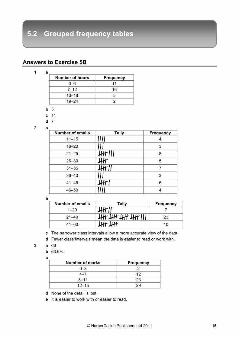
1 a Number of hours Frequency

0–6 11

7–12 16

13–18 5

19–24 2

b 5

c 11

d 7

2 a Number of emails Tally Frequency

11–15 4

16–20 3

21–25 8

26–30 5

31–35 7

36–40 3

41–45 6

46–50 4

b Number of emails Tally Frequency

1–20 7

21–40 23

41–60 10

c The narrower class intervals allow a more accurate view of the data.

d Fewer class intervals mean the data is easier to read or work with.

3 a 66

b 63.6%.

c Number of marks Frequency

0–3 2 4–7 12 8–11 23 12–15 29

d None of the detail is lost.

e It is easier to work with or easier to read.


Lesson 5.2: Grouped frequency tables

4 a Height (h) in cm Frequency

140 ≤ h < 150 4 150 ≤ h < 160 8 160 ≤ h < 170 5 170 ≤ h < 180 3

b 8

c 4

d 170 ≤ h < 180 cm.

5 a Masses (m) in kg Frequency

45 ≤ m < 50 3 50 ≤ m < 55 4 55 ≤ m < 60 4 60 ≤ m < 65 5 65 ≤ m < 70 3 70 ≤ m < 75 4

b 11

c 55 ≤ m < 60 kg.

6

Pocket money (euros) Tally Frequency

5.00–7.99 6

8.00–10.99 9

11.00–13.99 7

14.00–16.99 2

7 a

Weight w (nearest gram) Tally Frequency

20 ≤ w < 25 4

25 ≤ w < 30 4

30 ≤ w < 35 2

35 ≤ w < 40 3

40 ≤ w < 45 5

45 ≤ w < 50 1

50 ≤ w < 55 1

b 8 books.

c 40 ≤ w < 45.


Lesson 5.2: Grouped frequency tables

d Weight w (nearest gram) Tally Frequency

20 ≤ w < 30 8

30 ≤ w < 40 5

40 ≤ w < 50 6

e There is a data point missing as the final range does not include it (52 g). The first table gives a better representation of the original data and patterns are easier to see.

8 a i 19.5 minutes.

ii 24.5 minutes.

b To capture the extreme values that lie greater than 50 minutes.

c When the data is not evenly spread across the range, class intervals of varying width are more useful.

d Yes, there is support for her belief as 31

25 students (81%) completed the homework in

less than 35 minutes.


5.3 Two-way tables

Answers to Exercise 5C

1 a 1

b 19

c 32

d They had no sausages or toast with their breakfast.

2 a 1

b 7

c 6

d Ginger / auburn.

e 30

f 6.7% (1 d.p.).

3 a 3

b 6

c 15

d 10%.

4 a

RS German History Total

Female 35 5 13 53

Male 12 17 18 47

Total 47 22 31 100

b 18

c 5

d 31

e 35%.

5 a

School lunch Packed lunch Other Total

Female 17 9 6 32

Male 21 7 0 28

Total 38 16 6 60

b 9

c 0

d 16

e 10

1


Lesson 5.3: Two-way tables

6 a

Male Female Total

Watched football 21 24 45

Did not watch football 8 8 16

Total 29 32 61

b 8

c 16

d 72.4%.

7 a 12%.

b East.

c Due to rounding of the figures.


6.1 Pictograms, line graphs and bar charts


1 a

b Southampton.

c 11 days.

2 a

b There would be too many symbols and it would be hard to read off the values.


Lesson 6.1: Pictograms, line graphs and bar charts

3 a

b For example; drivers heard about the speed trap and slowed down.

c Bar chart easier to read accurately.

4 a

b No. The number of speeders keeps changing.

5 Bar chart. It allows the easiest comparison of the number of cars caught speeding per day.



6 a

b Easy to draw, can show 50 easily, easy to see which day most burgers were sold.

7 Answers might include: last day, so more people there; colder weather; other food vendors had left or run out of food.

8



9 a

b No. The burger van will be somewhere else next Saturday as the music festival has finished.

10 a Carnations.

b Roses.

c 35

d 30

11 a 17

b

c 50 texts.


6.2 Pie charts


1

2

3 a 45°

b 20 people.

4 23.9 cm.

5 a The proportion of elm trees has been reduced dramatically.

b The pie charts show the proportion of trees in 1955 and 1995. If the total number of trees is the same, then the number of beech trees will have increased. However, as it does not state that these are comparative pie charts, this cannot be assumed. The total number of trees could now be smaller. The pie charts show that the proportion of beech trees is greater, but they do not show that the number of beech trees has increased.


6.3 Misleading graphs


1 a The y-axis starts at 60, which makes the most popular type (films) look almost twice as popular as cartoons, when in fact there is only a small difference of 15 between them.

b

2 There is no vertical scale, so we don’t know what the increase in petrol price is.

3 The graph’s y-axis starts at 1.0 rather than 0, and the years 2005–2008 have been missed out on the x-axis.


Lesson 6.3: Misleading graphs

4 a

b The y-axis starts at 15, which makes the busiest day (Saturday) appear to have sold many time more shoes than the quietest day (Wednesday). In reality, Saturday’s sales were 2.5 times those on Wednesday.

5 a

b By starting the y-axis at 190000 litres, it makes it appear that no petrol was sold on Thursday.

6 Due to the angle that the pie chart is being viewed from, it looks as though the sector at the front (the 'week after') is much larger than the other two. It is misleading because we cannot clearly see judge the proportional size of the three sectors.


6.4 Choropleth maps

Answers to Exercise 6D

1 a Italy

b 3.1–4.0 car thefts per 1000 people.

c There are 12 countries showing between 0.0 and 1.0 stolen cars per 1000 people. It would be better to split this group into two groups. Also, the choice of colours could be improved as they are many similar shades which reduces the ability to differentiate the areas on the map.

2 a

b See red line on diagram.

c This area of the reef has lower fish numbers than the rest of the coral reef.

d See blue line on diagram.

e This area of the reef has higher fish numbers than the rest of the coral reef.

3 a

b See red line on diagram.

c Without trees in these areas, there will be fewer birds.

d See blue line on diagram.

4 a Aberdeen City and City of Edinburgh.

b These two cities must have had a lot of people moving to them during this time for work or education.

c 0%

d There are many regions shown in the same colour. It would be better to have more shades to differentiate between these areas, e.g. the regions could be split into 0%, 0.1%, 0.2%, 0.3%, etc.


Lesson 6.4: Choropleth maps

5 a

b See red X on diagram.

c No one is standing near there.

d See blue arrow on diagram.

e Fewer people in this direction.

6 a

b There are very few nests around the edge of the forest. Most of the nests are near the centre of the forest.


6.5 Stem-and-leaf diagrams

Answers to Exercise 6E

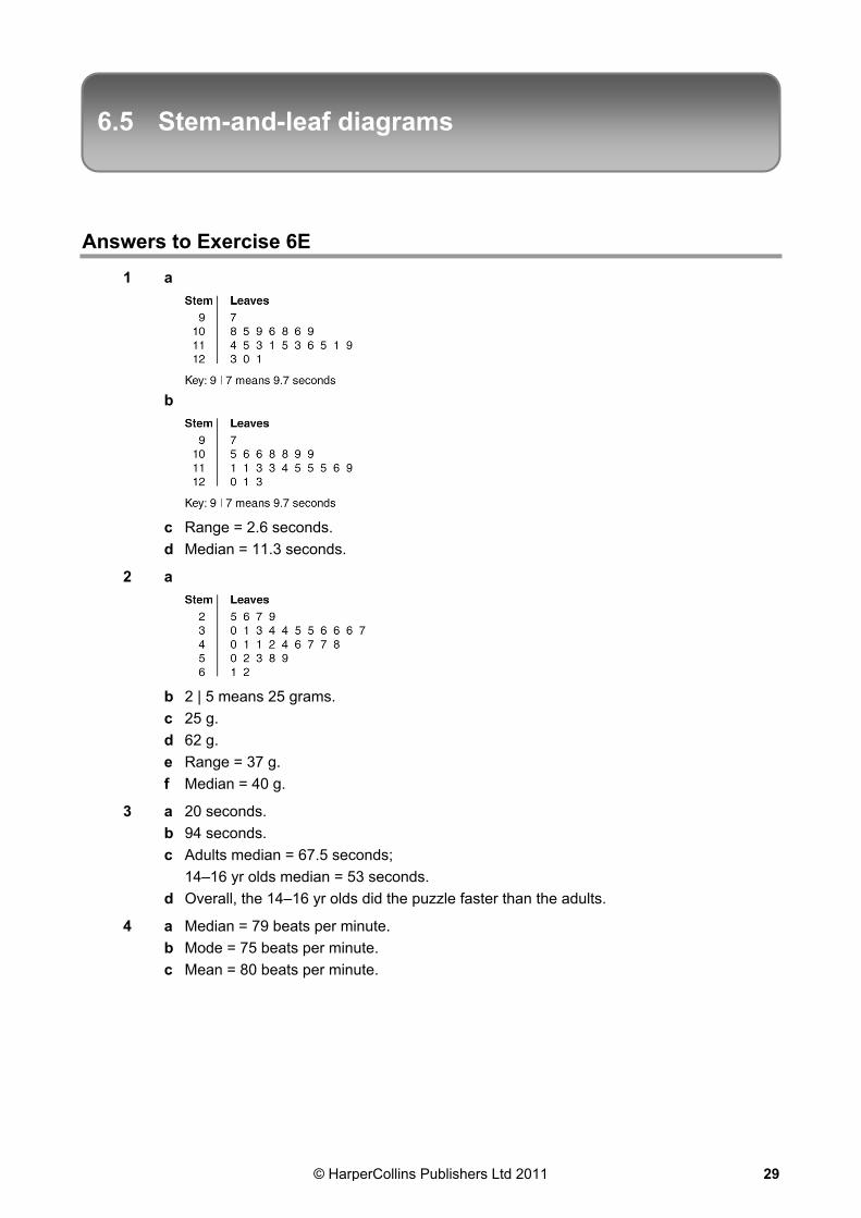
1 a

b

c Range = 2.6 seconds.

d Median = 11.3 seconds.

2 a

b 2 | 5 means 25 grams.

c 25 g.

d 62 g.

e Range = 37 g.

f Median = 40 g.

3 a 20 seconds.

b 94 seconds.

c Adults median = 67.5 seconds;

14–16 yr olds median = 53 seconds.

d Overall, the 14–16 yr olds did the puzzle faster than the adults.

4 a Median = 79 beats per minute.

b Mode = 75 beats per minute.

c Mean = 80 beats per minute.


6.6 Histograms and frequency polygons

Answers to Exercise 6F

1 a, b

2 a

b 77% of the sample are aged below 35 and they would be unlikely to enjoy an article on buying antiques. However, the subject matter of the magazine is unknown and the article might be relevant to the readers so their age might not be a significant factor.


Lesson 6.6: Histograms and frequency polygons

3 That is the middle value of the age group 0 to 10. It would be very unusual for most of them to be exactly in the middle at 5 years old. Also, if you added up the number of other runners, the total is 55 – much more than the 25 in the 0 to 10 group which is the modal class.

4 a

Mass, m Tally Frequency

10 ≤ m <12 8

12 ≤ m <14 6

14 ≤ m <16 13

16 ≤ m <18 10

18 ≤ m < 20 5

b

c 14 ≤ m <16.

d 14 ≤ m <16.



5 a

b 26 students.

6 a

Distance (miles) 7–10 10–13 13–14 14–15 15–17 17–20

Frequency 9 21 18 17 17 18

b 50.5% of cars.



7 a

Distance (km) 3–6 6–9 9–10 10–11 11–13 13–16

Frequency 18 42 36 34 34 36

Frequency density 6 14 36 34 17 12

b, c

d 77%.


6.7 Cumulative frequency graphs

Answers to Exercise 6G

1 Interquartile range = 45 – 30 = 15%.

2 a

b Median = 54

c Interquartile range = 72 – 42 = 30

d 17

140

e 140

2215.7% (1 d.p.)


Lesson 6.7: Cumulative frequency graphs

3 a

b 3

c 1

4 11 to 14 seconds.

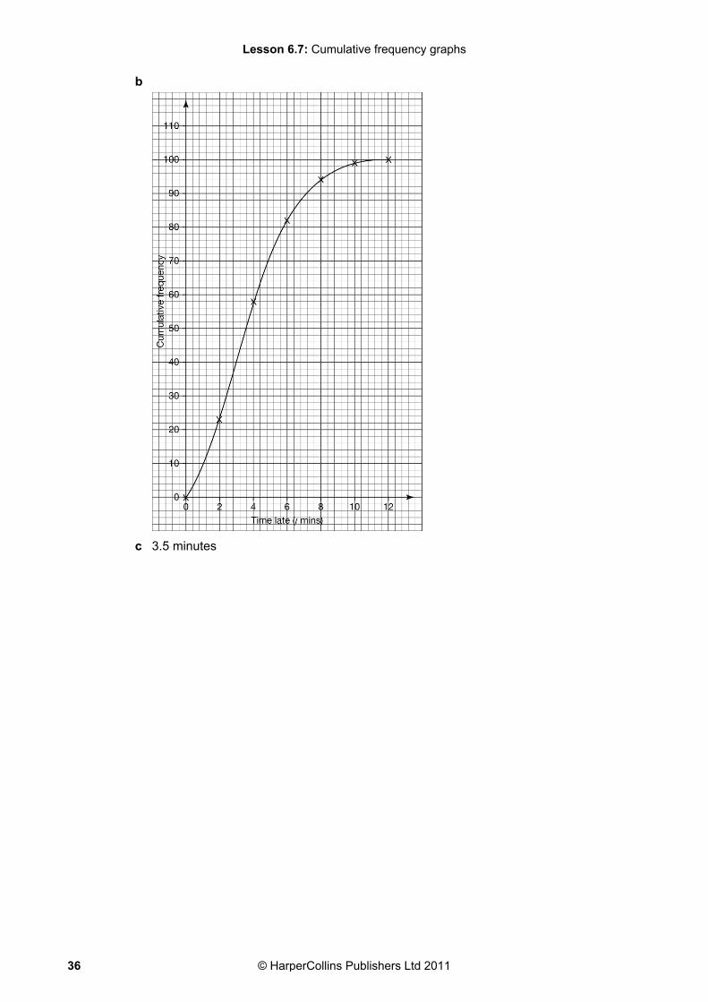
5 a

Time late (t mins) Cumulative frequency

0 ≤ t ≤ 2 23

2 < t ≤ 4 58

4 < t ≤ 6 82

6 < t ≤ 8 94

8 < t ≤ 10 99

10 < t ≤ 12 100


Lesson 6.7: Cumulative frequency graphs

b

c 3.5 minutes


7.1 The mode


1 a 4

b 5

c 6

2 0

3 86p.

4 A.

5 Seat.

6 a 3

b 10

c 20

7 1 goal.

8 3 bedrooms.

9 2, 4, 4.

10 4, 4, 4, 5, 5, 8.

11 75 g.

12 12 ≤ h < 14.


7.2 The median


1 a 5

b 4

c 7

d 12

e 3.9

2 a Mode = £7.99

b Median = £6.50

3 a 4

b 3.5

4 a Mode = 25

b Median = 22.5

5 a 3

b 20

c 17.5

6 a Mode = 0 goals.

b Median = 1 goals.

7 a 24 tables.

b Mode = £49.

c Median = £47.50

8 The first three must be 4, 4, 6. The other numbers must be bigger than 6, as 6 is the median, but they cannot be either 6 or the same number as each other as the mode is 4.

9 They must add up to £13.

10 a Median of Region A = 6.

b Median of Region B = 7.

c Region B is nearest. It has many more nests and a higher median number of eggs per nest.

11 a Mode = 1412

inches.

b Median = 15 inches.

c Mean = 14.85 inches.

d Either mode as most shirts were this size, or median as it’s the middle value best describe the data. Mean is less preferred at its value does not fall into one of the discrete shirt sizes.


7.3 The mean


1 a 5

b 6

c 6.8

d 12

2 a Mean = 24 friends.

b Mode = 20 friends.

c Median = 20.5 friends.

3 a Mean = 53 boys.

b Mean = 54 girls.

c Mean = 107 pupils.

4 a i Mean = 5

ii Mode = 3

iii Median = 4

b i Mean = 7

ii Mode = 9

iii Median = 8

c i Mean = 3

ii Mode = 2

iii Median = 2.5

5 a 28 conkers.

b 30 conkers.

c 6 conkers.

6 91°F.

7 a 5.7

b 58

c 31

8 2.15 texts.

9 a Mean = 3.5 people.

b Mode = 2 people.

c Median = 3 people.

10 5.8 eggs (to 1 d.p.)


7.4 Which average to use


In all of these questions, when the best average has to be chosen, alternatives to these answers may be accepted if the reasons support them.

1 a i Mean = 7.67

ii Mode = 2

iii Median = 9.5

Median (9.5) probably represents data best, because there are two small items (2s) which make the mean and mode too small.

b i Mean = 8.57

ii Mode = 19

iii Median = 6

Median (6) probably represents data best, because there are two large items (19s) which make the mean and mode too large.

c i Mean = 13.75

ii Modes = 1 and 20

iii Median = 17

Median (17) probably represents data best, because there are two modes and there are two small items (1s) which make the mean too small.

2 a Mode is the only possible average because this is a qualitative variable.

b There may be some extreme values, making the mean not suitable. This is a continuous variable, so there may not be a mode, just lots of different values. The median is probably the best.

c The mean may be best here because we want to make sure every piece of data is included.

3 a Mode = £8000

b Median = £24 750

c Mean = £28 200

The two £8000s make the mode too small, and the very large £90 000 makes the mean too big, so the median is probably best.

4 a Mode = 4 people.

b Median = 3.5 people.

c Mean = 3.25 people.

Mode is most useful to the builder, because he can build his houses to fit this size of family and maximise his potential market.

5 a Mode = 15 years.

b Median = 15 years.

c Mean = 17.5 years.

The mean is not suitable, because the age of the teacher is so much more than the pupils’ ages that it makes the mean too big.


Lesson 7.4: Which average to use

6 a Mode = £0

b Median = £5

c Mean = £16.25

The mean is the most suitable as all values need to be included.

7 The data is qualitative not quantitative, so we can only find the mode.

8 a There is no mode.

b Median = 10 errors.

c Mean = 12.8 errors.

The median best describes the data. The mean is badly affected by the 45, giving a value bigger than most of the data. There is no mode.

9 a i Mean = 36.05 chocolates.

ii Median = 38 chocolates.

iii Mode = 40 chocolates.

b i The mean will go up, but the median and mode will not change.

ii It looks as if the manufacturer is using the mode, because this represents the most common amount of sweets found in a sample.

10 a Mr Truman’s PE class: mean = 32, mode = 47, median = 31.

Median, as the 7 could be seen as extreme data and the mode is too high.

b Mr Thom’s PE class: mean = 32.9, mode = 33, median = 33.5.

Mean, as there is no extreme data.

c Mr Thom’s PE class as higher mean and median distance and are more consistent.


7.5 Grouped data


1 a

Time taken, x, (seconds)

Number of people

Mid-point value

20 ≤ x < 30 18 25 450

30 ≤ x < 40 12 35 420

40 ≤ x < 50 6 45 270

50 ≤ x < 60 24 55 1320

Total 2460

b Estimate of the mean = 41 seconds.

2 a Estimate of the mean = 11.3

b Estimate of the mean = 25

c Estimate of the mean = 14.8

3 a Modal class = 0 < x ≤ 20

b Estimate of the mean = £32.67

4 Estimate of the mean = £122.50

5 a Modal class = 2 < t ≤ 4

b Estimate of the mean = 3.68 hours.

6 a Modal class = 8 < t ≤ 12

b Estimate of the mean = 8.8 minutes.

7 Estimate of the mean = 207 pages.

8 Estimate of the mean = 49.7 marks (to 1 d.p.)

9 Estimate of the mean on Day 1 = 24.25 seconds.

Estimate of the mean on Day 2 = 21 seconds.

So the estimate of the mean is lower by 3.25 seconds on Day 2.

10 18


7.6 The geometric mean


1 a 8

b 2.01

c 6

d 4.22

e 6.31

f 8.81

2 a 1.04

b 1.03

c 1.12

d 1.025

e 0.95

f 0.87

3 504.1 = 1.2167 = +21.7%.

4 4 97.005.102.104.1 = 1.01953 = +1.95%

5 +7.88%

6 +7.15%

7 +24.82%

8 +6.2%

9 72.0y64.0 , y = 64.0

72.0 2

= 0.81; Price fell by 19% in the second year.

10 3, 24, 24


8.1 Box-and-whisker plots


1 a

b

c

2 a

b The men’s median age is bigger, which shows they are older on average. The men’s interquartile range is bigger, showing their ages are more spread out than the women’s ages. The men’s ages are negatively skewed and the women’s are positively skewed, showing that most of the men are older than most of the women.

3 a


Lesson 8.1: Box-and-whisker plots

b White’s median price is bigger, which shows the cars there are more expensive on average. Green’s interquartile range is bigger, showing that their prices vary more than White’s prices. Green’s prices are negatively skewed and White’s are positively skewed, showing that some of Green’s cars are cheaper and that some of White’s cars are more expensive, comparatively.

4 a

b Both distributions are symmetrical and have the same median, so the two resorts have the same number of hours sunshine on average. However, Resort B has a bigger interquartile range, so the hours of sunshine there vary more. It has the days with most sunshine, but also the days with least sunshine.

5 No. There will probably be a few who get very little or even no pocket money, lots who get around the same amount and a few who get a lot of pocket money.

6 a

b Median = 52 marks.

Upper quartile = 64 marks.

Lower quartile = 39 marks.


Lesson 8.1: Box-and-whisker plots

c

7 a The top box plot is for Granada, as the mountains would get colder than the beach in September.

b The top box plot has much lower minimum temperatures, a lower LQ, a lower UQ and a much bigger range and interquartile range. Both box plots have the same median and highest temperature.

8 a

Lowest value 22

Lower quartile 28

Median 33

Upper quartile 38

Highest value 55

b LQ 1.5 × IQR = 13, so no low outliers.

UQ + 1.5 × IQR = 53, so 55 is an outlier.

c

9 A = Q, B = R, C = S, D = P


8.2 Variance and standard deviation


1 a 2.55

b 5.74

c 4.08

2 a Mean = 59.2 marks.

b Standard deviation = 14.8 marks.

3 a 0.92

b 2.14

c 6.31

4 a Mean = 2.05 pets.

b Variance = 1.40

c Standard deviation = 1.18

5 a Mean = 2.22 televisions.

b Variance = 1.52

c Standard deviation = 1.22

6 a Mean = 7.07 books.

b Variance = 1.03

7 a Estimate of the mean = 9.26 kg.

b Estimate of the variance = 14.4

8 a Estimate of the standard deviation = 4.43

b Estimate of the standard deviation = 12.1

c Estimate of the standard deviation = 6.28

9 Estimate of the standard deviation = 15.9 cm.

10 Variance = 7.38

11 a Estimate of the mean = 42 minutes.

b Estimate of the standard deviation = 8.06

12 Yes, within this population 88.1% weigh between 750g and 1.5 kg.


8.3 Properties of frequency distributions


1 a

b Positive skew.

2 a

b Both distributions are symmetrical, so mean = median = mode. Group B is the better at

running the 400 m than Group A. Group B have a mean time of 55 seconds, while Group A’s mean time is 65 seconds. Group B’s distribution is much narrower than Group A’s, which shows that Group B has more consistent times than Group A.

3 a Symmetrical

b Negatively skewed

c Positively skewed

d Symmetrical

e Positively skewed


Lesson 8.3: Properties of frequency distributions

4 a 0

b –0.5

c 0.67

d 0

e 1.33

5 a

b Symmetrical, not skewed.

c Normal distribution.

6 a i 4.39

ii 4

iii 0.920

iv 0.424

b i 7.27

ii 6

iii 2.39

iv 0.531

c i 15.6

ii 15

iii 6.71

iv 0.0894

7 a 40 to 160

b 60 to 140

c 80 to 120


Lesson 8.3: Properties of frequency distributions

8 a

b The rugby players had a greater spread of results and a higher mean than the footballers. 68% of the rugby players weigh between 70 and 100 kg, whereas 68% of the footballers weigh between 66 and 86 kg.

9 180 + (2 × 40) = 260 seconds and 180 – (2 × 40) = 100 seconds, so 95% of people queue between 1 minute 40 seconds and 4 minutes 20 seconds.

10 a Standard deviation = 8 seconds.

b Between 51 and 99 seconds.

11 a 1

b 2

c –1

d –1.5

e 0

f 0.25

12 a 80

b 88

c 40

d 84

e 48

13 0.1%.

14 Standard deviation = 4.5 cm.


9.1 Statistics used in everyday life


1 a 91.4

b 58.9

c 41 1% reduction.

d 1 119 990 tonnes.

2 a £1 = 1.10 Euros

b January and February

c There is no trend in the data.

3

Year 2005 2006 2007 2008 2009 2010

Index 100 112 132 144 135 142

Price £2.84 £3.18 £3.75 £4.09 £3.83 4.03

4 a Weighted index = 138.0

b Labour

5 a 2008 – 2009 = 105.6

2009 – 2010 = 122.5

b From 2008 to 2009 her car insurance rose by 5.6%, whilst from 2009 to 2010 her car insurance rose by 22.5%.

c Answers might include: She bought a new car, added other people to her insurance; had a crash or received points on her driving licence.

6 General cost of living in 2010 rose 31% compared with 2000.

7 In this town, 8.3 people per 1000 die per year when weighted according to the national standard population.


10.1 Time series and moving averages


1 a 08:00

b 16°C

c 16:00 and 20:00

d 11.5°C

e 9 hours.

2 a

b 61

c The trend is increasing. He is getting better at the questions being asked in the quiz.

d It is unlikely that his scores will keep increasing. His score cannot pass 100.


Lesson 10.1: Time series and moving averages

3 a

b Estimate of £18–£19 billion.

c The trend is increasing; more money is being spent by tourists in the UK each year. This could be due to people have more money to spend, more tourists, higher prices.

d Due to the London 2012 Olympics.

4 a From 1997 to 2000 there is a slight increase in the number of barn owl eggs hatched. Then there is a large increase in 2001, and from 2001 to 2004 the numbers increase slowly again. The number stayed the same from 2004 to 2005.

b 12.5 ± 0.5 eggs.

c Not reliable; 2011 is too far from the rest of the data.

5 a

b 20 ± 1 goldfish.

c 2005 and 2006.

d For example, the pond is getting full up with fish, there is insufficient food, there is a predator living in the pond.

e No, there are too many unknowns in the future for prediction to be possible.



6 a

b £159 000 ± 2000

c People want to live near the sea, so the prices are higher as you get nearer the sea.

d No. The prices would not keep going down just because the flat was further away from the seafront.

7 a (134 + 78 + 52 + 120) ÷ 4 = 96

b 106.5, 108.5, 108.75

c



d £22 to £24

e £135 to £140

8 a Cumulative totals from March: 4500, 5700, 7000, 8350, 9750, 11 000, 12 150, 13 400, 14 650, 15 900

b

c They are reducing steadily over time.



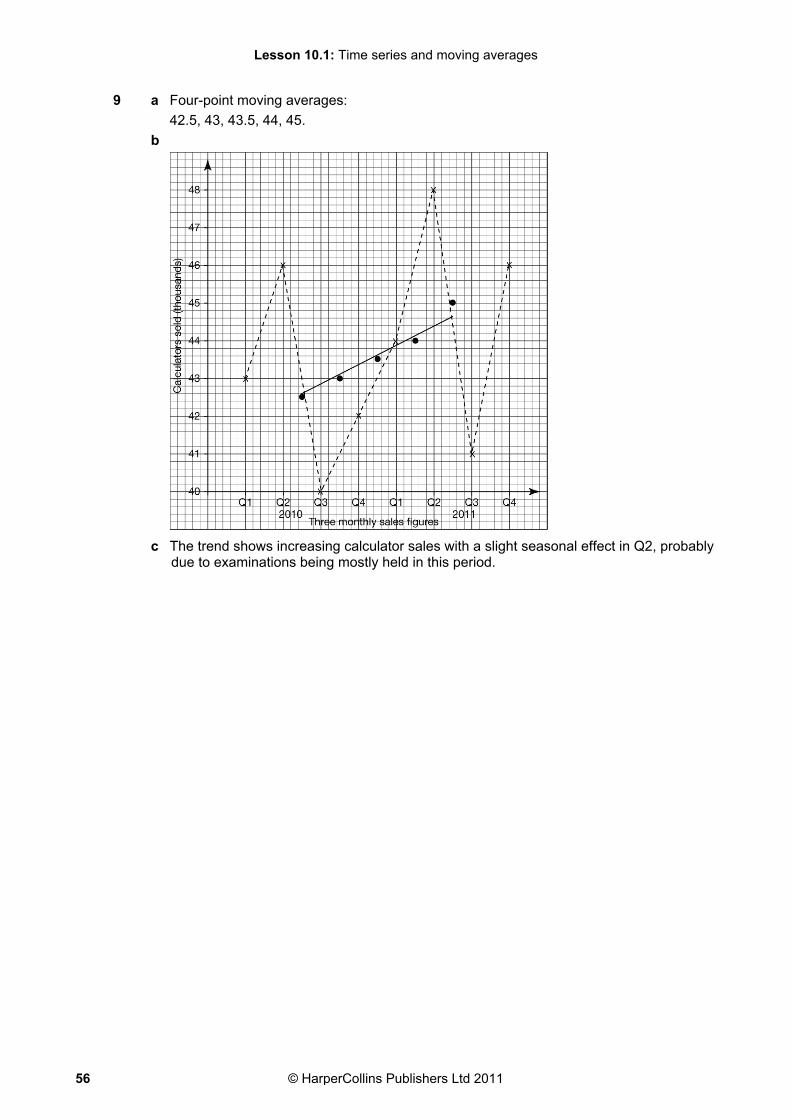
9 a Four-point moving averages:

42.5, 43, 43.5, 44, 45.

b

c The trend shows increasing calculator sales with a slight seasonal effect in Q2, probably due to examinations being mostly held in this period.


10.2 Quality assurance


1 a Mean = 20.0 kg

b Median = 20.0 kg

c Yes, both give the average weight per bag, but neither shows the spread of weights and that half of the bags are underweight.

d The range: this would show that the weight per bag is inconsistent.

2 a Mean = 10.2 litres.

b Median = 10.0 litres.

c Although both measures give the average capacity per bag, neither shows the spread of capacity and that half of the bags are underweight.

d Yes, the machines should be much more consistent.

3 a 501.58 g.

b Yes – the mean is above 500 g.

c The 499.7 g and the two 499.6 g boxes could pose a problem. Alert/vigilant consumers could complain and possibly sue the company for being short-changed. They could refuse to buy that brand again or give the company a bad reputation.

4 a 31.32 ml.

b Although the mean and median are over 30 ml, this is quite a small sample. More data would be required.

c Improve the consistency of filling the bottles. Be careful, as 1 in 5 (20% of sample) did not have enough oil in the bottle.

5 a 401.3 g.

b Yes, the mean is more than 400 g.

c Yes, one box is underweight; it is illegal to do this.

6 a 19.19 g.

b No.

c Possibly. The sample mean is dropping at each sample.

d Reset the machine.

e No. It would be better to take random samples or one packet for every 800 packets packed.


Lesson 10.2: Quality assurance

7 a Upper limit = 193.92 g; lower limit = 190.08 g.

b, c

d Yes, one of the sample means is not within acceptable limits for the machine.

8 a

b Yes: there are packs which contain less than 150 toothpicks and the range is outside of acceptable limits in two out of five samples taken.

c Analyse more samples and reset the machines that count out the toothpicks if required. Continue to analyse the containers to ensure the corrective action has been effective.


11.1 Scatter diagrams and correlation


1 a Positive correlation – the expected result would be for shoe size to increase as height increases.

b No correlation – the expected result would be that no correlation exists.

c Positive correlation – the expected result would be ability in maths is related to ability in science.

d No correlation – the expected result would be that no correlation exists.

e Negative correlation – the expected result would be that the more money spent on downloads, the less money is saved.

2 a, c

b Mean height 1.77 m; mean weight 74.4 kg.

d 67.2 kg.


Lesson 11.1: Scatter diagrams and correlation

3 a, c

b Mean breaths per minute 26.2; mean pulse beats per minute 80.

d 93 pulse beats.



4 a, b

b Mean age 14.45; mean height 1.76 m.

c Misca’s estimated age = 14.3 years.

d People do not keep growing at the same rate once pass their teenage years.



5 a, b

b English mean = 51; history mean = 48.

c Jamir. He was a long way from the line of best fit. He should have got around 71 marks.

d Brian. He was a long way from the line of best fit. He should have got around 56 marks.

e 64 marks.

6 a, c

b Reading mean = 2.4 bar; correct reading mean = 3.36 bar (to 3 s.f.).



d y = 1x + 1 (exact answer dependent upon line of best fit – allow 10% either side).

e The correct tyre pressure when there is no reading on the gauge.

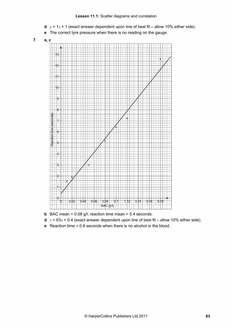
7 a, c

b BAC mean = 0.08 g/l; reaction time mean = 5.4 seconds.

d y = 63x + 0.4 (exact answer dependent upon line of best fit – allow 10% either side).

e Reaction time = 0.8 seconds when there is no alcohol in the blood.


11.2 Spearman’s rank and product moment correlation coefficients


1 a Hours of sunshine vs. amount of rain: very strong negative correlation (the more hours of sunshine, the less rain).

b Size of diamond vs. price of diamond: strong positive correlation (the bigger the diamond, the more it costs).

c Eye colour vs. height: weak positive correlation (there may or may not be a relationship between eye colour and height).

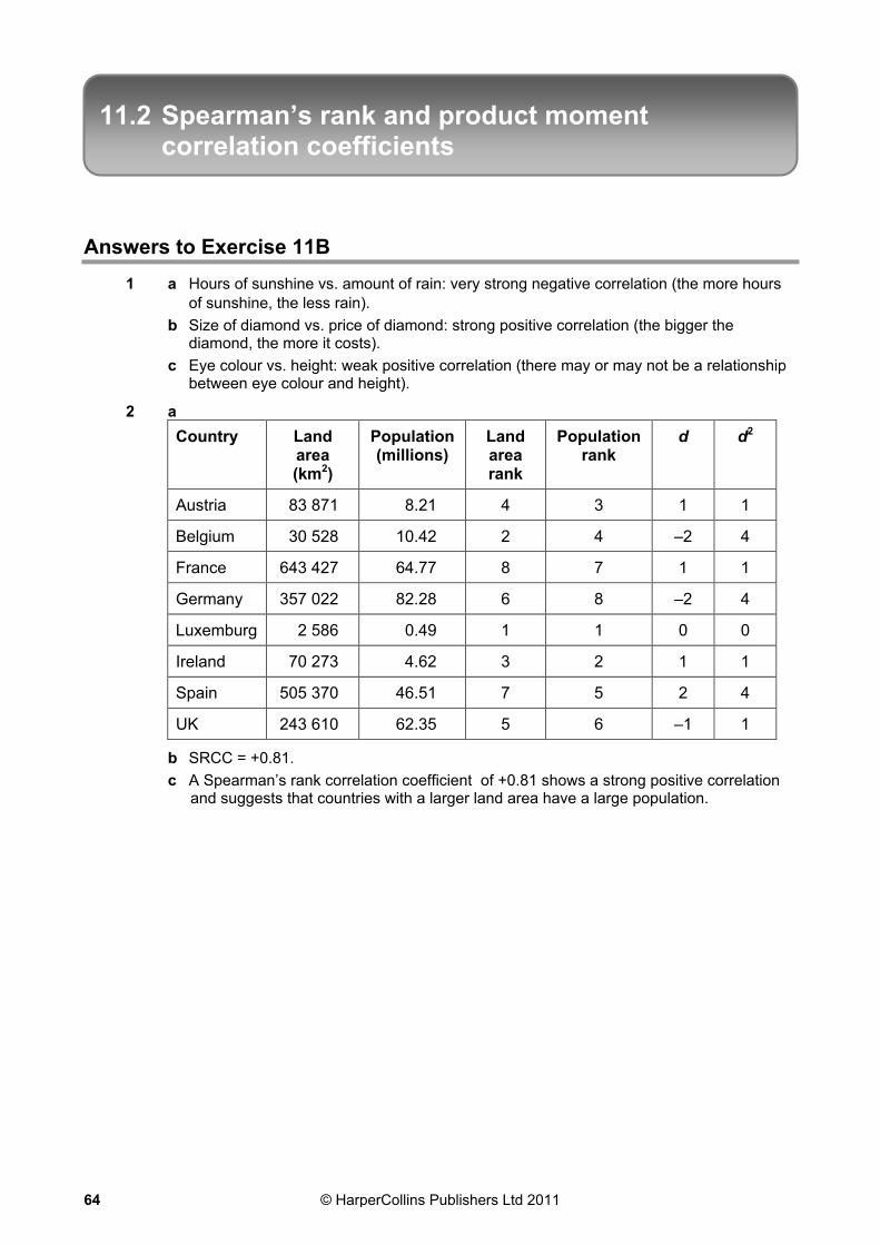
2 a

Country Land area (km2)

Population (millions)

Land area rank

Population rank

d d2

Austria 83 871 8.21 4 3 1 1

Belgium 30 528 10.42 2 4 –2 4

France 643 427 64.77 8 7 1 1

Germany 357 022 82.28 6 8 –2 4

Luxemburg 2 586 0.49 1 1 0 0

Ireland 70 273 4.62 3 2 1 1

Spain 505 370 46.51 7 5 2 4

UK 243 610 62.35 5 6 –1 1

b SRCC = +0.81.

c A Spearman’s rank correlation coefficient of +0.81 shows a strong positive correlation and suggests that countries with a larger land area have a large population.


Lesson 11.2: Spearman’s rank and product moment correlation coefficients

3 a

Athlete 5000 m 10 000 m 5000 m rank

10 000 m rank

Difference d

d2

A 15.36 31.34 5 6 –1 1

B 16.55 32.33 8 7 1 1

C 13.50 30.02 1 4 –3 9

D 14.25 29.44 2 2 0 0

E 17.32 38.23 9 10 –1 1

F 20.12 36.40 10 9 1 1

G 14.48 29.57 3 3 0 0

H 15.45 30.09 6 5 1 1

I 14.58 28.52 4 1 3 9

J 16.04 32.35 7 8 –1 1

b Σd2 = 24, n = 10, SRCC = +0.85.

c +0.85 shows strong positive correlation and suggest that athletes who have fast 5000 m times also have fast 10 000 m times. The reverse is also true.


Lesson 11.2: Spearman’s rank and product moment correlation coefficients

4 a

Month Rainfall (mm)

Sunshine (hours)

Rainfall rank

Sunshine rank

Difference d

d2

January 1.36 1.2 3 12 –9 81

February 1.35 2.7 2 10 –8 64

March 0.75 4.6 1 7 –6 36

April 2.22 5.2 8 4.5 3.5 12.25

May 2.54 5.7 10 3 7 49

June 2.26 7.7 9 1 8 64

July 2.99 5.2 12 4.5 7.5 56.25

August 1.84 5.8 6 2 4 16

September 2.66 4.9 11 6 5 25

October 1.74 3.1 5 8 –3 9

November 1.57 2.9 4 9 –5 25

December 2.09 1.9 7 11 –4 16

b Σd2 = 453.5, n = 12, SRCC = –0.59.

c –0.59 shows a fairly strong negative correlation and suggests that the more rain there is, the less sunshine there is. The reverse is also true.

5 a SRCC = +0.75.

b +0.75 is a fairly strong positive correlation, so the judges mainly agree on who is the best (and worst).

6 SRCC = +0.63.

There is some positive correlation between the marks, so Alicia is probably correct.

7 SRCC = +0.83.

There is strong positive correlation, so the longer a person smokes, the worse their lung damage is likely to be.


12.1 Probability scale


1

Word Probability

Even chance 0.5

Certain 1

Likely 0.8

Impossible 0

Unlikely 0.25

2 Impossible, very unlikely, even chance, likely, very likely, certain.

3 a 1

b 0

c 0.5

4 a Very likely

b Very unlikely

5 a Impossible

b Even chance

c Certain

d Likely

e Unlikely

6 a, b

7 a, b, c

8 Ali said that it might rain or that it might not rain. This doesn’t mean that there is an even chance of rain as Ali doesn’t consider the probability of it raining. For an even chance, the probability of rain = probability of no rain = 0.5.


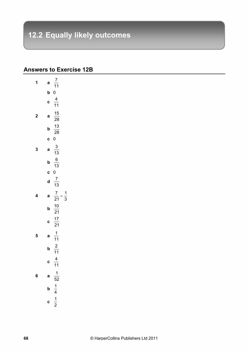
12.2 Equally likely outcomes


1 a 11

7

b 0

c 11

4

2 a 28

15

b 28

13

c 0

3 a 13

3

b 13

6

c 0

d 13

7

4 a 3

1

21

7

b 21

10

c 21

17

5 a 11

1

b 11

2

c 11

4

6 a 52

1

b 4

1

c 2

1


Lesson 12.2: Equally likely outcomes

d 13

1

52

4

e 13

12

52

48

7 a 1000

3

b 50

1

1000

20

c 1000

21

d 250

247

1000

988

8 1213

9 0.4

10 0.8

11 0.28

12 411


12.3 The addition rule for events


1 a 13

7

b 13

1

c 13

6

d 13

12

e 6

13

2 a 12

5

b 3

1

12

4

c 3

2

12

8

d 1

3 a 10

3

b 5

1

10

2

c 5

2

10

4

d 10

3

e 10

7

4 a 52

1

b 2

1

c 4

1

d 26

7


Lesson 12.3: The addition rule for events

e 52

27

5 a 11

3

b 11

6

c 11

3

d 11

9

6 Lucy, whose probability of winning is 0.45.

7 Jack since his probability is 5

2.

8

Type Probability Number of questions

Science and nature 0.4 6400

History and geography 0.25 4000

Literature, art and music 0.3 4800

Weird stuff 0.05 800


12.4 Experimental probability


1 a Equally likely outcomes.

b Historical data.

c Historical data.

d Survey or experiment.

2 a 6

1

b i 0.08

ii 0.09

iii 0.106

iv 0.105

v 0.1516

vi 0.168

vii 0.1655

c 2000

3 a

Number of times pin dropped

Number of times pin lands point up

Experimental probability

i 100 87 0.87

ii 200 148 0.74

iii 500 335 0.67

iv 1000 584 0.584

v 1500 883 0.5886

vi 2000 1182 0.591

vii 2500 1492 0.5968

viii 3000 1797 0.599

b 0.6

c 10 800

4 Wednesday

5 9990

6 She is wrong because the P(4) = 4

1since the ‘2’ occupies half of the spinner.

3004

1 is not 100. You would expect less than 100.

As it is an experiment she cannot predict how many ‘4’s she will get.


Lesson 12.4: Experimental probability

7 185 000

8 a The dice looks like it is biased towards a 4, since the relative frequency is much higher than the others and the expected probability of 20.

b Conduct the test with a greater amount of throws.

9 a 5

1

20

4 .

b Emily has spun the spinner more times so the results should be more reliable.

c 225.0120

27

10 a Bias

b No bias

c Bias


12.5 Combined events


1 12

1

2 a

Spinner 1

2 4 6 8

3 5 7 9 11

5 7 9 11 13

5 7 9 11 13

Spi

nner

2

7 9 11 13 15

b i 0

ii 4

1

16

4

iii 8

3

16

6

3 a

Dice 1

1 2 3 4 5 6

1 1 2 3 4 5 6

2 2 4 6 8 10 12

3 3 6 9 12 15 18

4 4 8 12 16 20 24

5 5 10 15 20 25 30

Dic

e 2

6 6 12 18 24 30 36

b i 4

1

36

9

ii 0

iii 9

1

36

4

iv 36

11

4 a 8

1

24

3

b 2

1

24

12


Lesson 12.5: Combined events

c 4

1

24

6

5 a 6

1

12

2

b 12

1

c 0

d i A six.

ii Probability = 3 1

=12 4

.

6 3

2

6

4

7 12

1

8 Probability of one five = 9 18

=50 100

. Probability of a total of five = 1 4

=25 100

.

Probability of a double five = 1

100. So for 100 people playing, Ishmael would payout

18 x £1 + 4 x £2 +1 x £10 = £36. This gives a 64% profit, so he will make money.


12.6 Expectation


1 8 days.

2 5 texts.

3 325

4 Red = 36 times; green = 18 times; yellow = 27 times.

5 18 days.

6 a 0.15

b 60

7 a 7

5

b 6

8 16

9 180

10 42

11 625

12 Probability of one ten = 9 18

=50 100

. Probability of a total of ten = 9

100.

Probability of a double ten = 1

100. So for 100 people playing, Katrin would expect to payout

18 x £1 + 9 x £5 +1 x £10 = £73. This gives an expected £27 profit, so she will make money.

13 139


12.7 Tree diagrams

Answers to Exercise 12G

1

a 8

3

16

6

b 2

1

16

8

2 a

b 36

1

c 36

10


Lesson 12.7: Tree diagrams

3 a

b 21

4

c 21

11

4 a

b 0.26

c 0.14

d 0.53

5 a

b 0.42

c 0.28

d 0.12


Lesson 12.7: Tree diagrams

6 a

b 0.32

c 0.56

7 a 0.28

b 0.18

c 0.54

8 a 33

14(assumes Kate does not replace her pen, before Richard chooses his.)

b 33

17

c 33

16

9 a 0.14

b 0.09

c 0.21

10 a 35

2

b 35

6

c 35

29

11 a 0.33915

b 0.18515

c 0.97345


12.8 Conditional probability

Answers to Exercise 12H

1 a

b 0.12

c 0.8

2 a

b 0.88

c 0.204

3 a 15

1

90

6

b 15

7

4 a 117

35

b 39

20

5 a 0.51

b 0.68


Lesson 12.8: Conditional probability

6 0.025

7 a 55

9

b 55

19

8 a 0.425

b 0.132

c 0.443


Real-life Statistics

Answers for Software developers

1

2

6 people play simulation and platform games.

3 People within games shops are likely to spend lots of time playing computer games. It is unlikely that a non-gaming person will be in there, so the survey results will be biased in favour of those who actually play games. She could improve her results by going to different venues at differing times and days to conduct her survey, which will result in a sample of people with different gaming habits.

Answers for Business consultants

1 Costing exercise:

– by what proportion would food/drink costs go up?

– would organic food change any other cost categories?

Survey current and potential customers on attitudes towards organic food:

– do they want organic food?

– would they be prepared to pay more?

2 Numerous answers including: inflation and/or pay rises; higher workload than forecast; absenteeism; poor productivity; expensive printing etc.

Office may miss bookings, make administration errors, poorly plan events etc.



3 Review the number of people employed against the size of the event (number of attendees). Analyse by using a scatter graph and line of best fit to predict the number of staff needed at future events.

Answers for Sports recruiters

1 To compare the data the best options are bar graphs or pie charts. Before doing this it is important to ensure the data is ready for comparison. The data is for all appearances made by the three players over the previous season. However, as they all played in differing number of games which has to be taken into consideration for most of the performance criteria.

The table below re-states the relevant performance data per appearance:

Players Fernando Joe Jamie Goals per game 0.53 0.64 0.62 Assists per game 0.28 0.64 0.32 Tackles made per game 1.39 8.00 4.05 Yellow cards per game 0.14 0.08 0.00 Red cards per game 0.08 0.04 0.00 Pass completion % 72 89 80

Using a composite bar graph helps to support the answer.

The coaches and manager belief they need an attacking player who can also play in

midfield. Therefore, goals, assists, tackling and passing are the most important data sets. From the composite bar graph, Joe is the best player for this position followed by Jamie.

There are two other factors for consideration – cost and fitness.

As the cost of each player is known, it is possible to consider the value for money each player represents. As Joe is the player with the lowest transfer price, this strengthens the support for his purchase.

However, as Joe played fewer games than the other two last season, it may be worthwhile ensuring that he is fully fit before purchasing.

2 The data available covers the last five seasons. As such, it is possible to use averages and measures of spread to represent the data. The mean should be used as it is important to use all the data. Standard deviation would probably be the best measure of spread although there are only five data points so range is an option.



The table below shows the calculated mean and standard deviation for each player:

Apps Goals Assists

2006/07 35 14 20

2007/08 27 12 13

2008/09 30 12 9

2009/10 32 26 11

2010/11 16 4 10

Mean 28 13.6 12.6

Wayne

SD 6.5 7.1 3.9

2006/07 36 20 3

2007/08 19 8 8

2008/09 24 5 5

2009/10 32 29 12

2010/11 24 10 10

Mean 27 14.4 7.6

Didier

SD 6.1 8.9 3.3

It would also be sensible to study the performance statistics per appearance. This can be done easily by using the mean data from the table above.

Wayne’s average goals per game 49.028

6.13

Didier’s average goals per game 53.027

4.14

Wayne’s average assists per game 45.028

6.12

Didier’s average assists per game 28.027

6.7

Finally, the data can be presented as a time series which will help to identify any trends over time.

The line graph below is an example of one of the graphs that could be used:

By comparing all the data with the most relevant calculations and methods, it has to be

concluded that the two players perform quite similarly.

Didier marginally outscores Wayne, but Wayne does contribute more in terms of assists.

The decision on who to sell may come down to other factors like the fact that Wayne is considerably younger than Didier and is the better long-term prospect.



Answers for Intelligence agencies

1 a Assign each area a number from 1 to 20. Use random number table to select an area or two (1 to 2 areas would give you a 5 – 10% sample size). From these areas, number the phones from 1 to 200, then use random number table to select a sample of 10 to 20. Test these phones to determine whether or not they fail.

b Probability = 0.63

Answers for Forensic scientists

1 Angle of entry of each bullet.

The depth of the bullet hole.

2 How tall were each of the robbers?

Where were the robbers standing when they fired their weapons?

How were the robbers holding their weapons when they fired them?

Answers for Marketing professionals

1 The most valuable data required is whether people own both cats and fish. This is missing from Daniel’s current research.

2 They might be the only people in the survey who own both cats and fish.

3 Do your pets include at least one cat and at least one fish?

Yes (please answer next question) No (please ignore next question)

Would you feed a new product 'cat food that can also feed your fish!' to your cat(s) and your fish?

Yes No Not sure


Documents

1.1 The data-handling cycle - Collins Educationresources.collins.co.uk/free/AQAGCSEStatisticsAnswers.pdf · b Students obtain higher marks if they take a maths exam in the ... inter-quartile