Embed Size (px)
Citation preview
11 January 2007 Constraints - Finite Domains 1
Constraints – Finite Domains
Advanced Constraints
• Cardinality Constraints
• Propositional Constraints
• Constructive Disjunction
Global Constraints
• Generalised Arc Consistency
• All-Different, Element, Circuit
11 January 2007 Constraints - Finite Domains 2
Cardinality (Meta-) Constraint
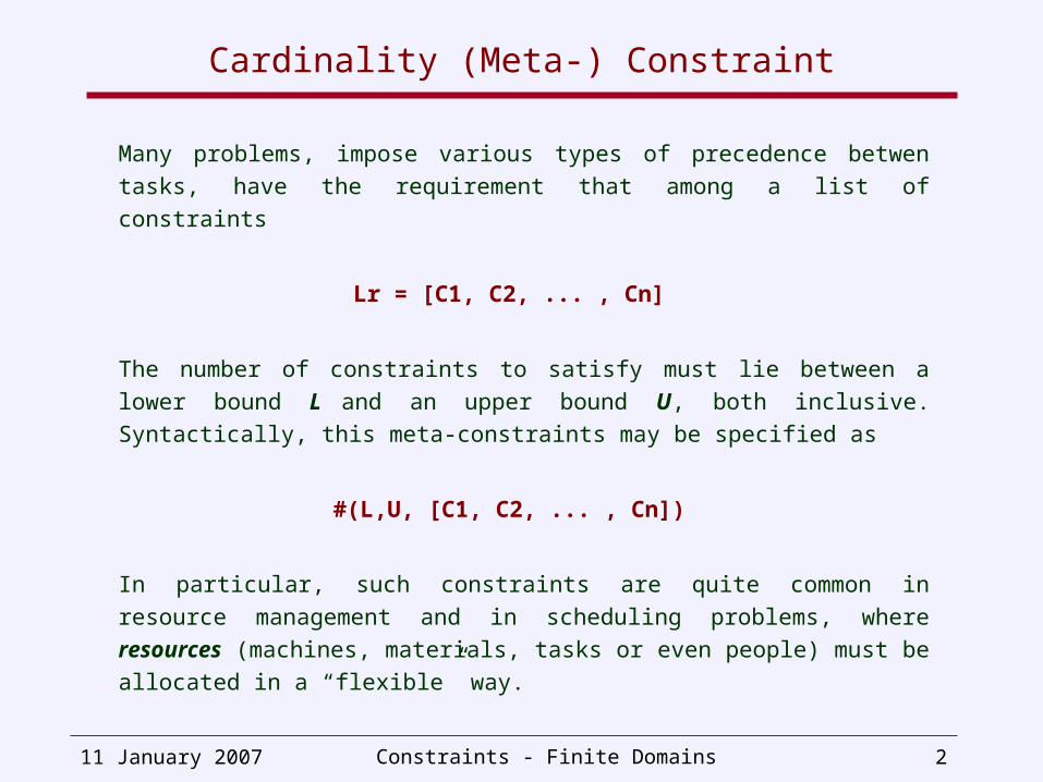
Many problems, impose various types of precedence betwen tasks, have the
requirement that among a list of constraints
Lr = [C1, C2, ... , Cn]
The number of constraints to satisfy must lie between a lower bound L and an
upper bound U, both inclusive. Syntactically, this meta-constraints may be
specified as
#(L,U, [C1, C2, ... , Cn])
In particular, such constraints are quite common in resource management and
in scheduling problems, where resources (machines, materials, tasks or even
people) must be allocated in a “flexible” way.
11 January 2007 Constraints - Finite Domains 3
Cardinality Constraint: Example
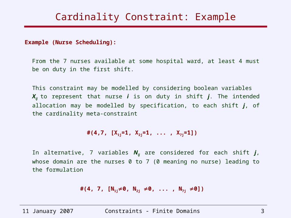
Example (Nurse Scheduling):
From the 7 nurses available at some hospital ward, at least 4 must be on duty
in the first shift.
This constraint may be modelled by considering boolean variables Xij to
represent that nurse i is on duty in shift j. The intended allocation may be
modelled by specification, to each shift j, of the cardinality meta-constraint
#(4,7, [X1j=1, X2j=1, ... , X7j=1])
In alternative, 7 variables Nij are considered for each shift j, whose domain are
the nurses 0 to 7 (0 meaning no nurse) leading to the formulation
#(4, 7, [N1j0, N2j 0, ... , N7j 0])
11 January 2007 Constraints - Finite Domains 4
Cardinality Constraint: Operational Semantics
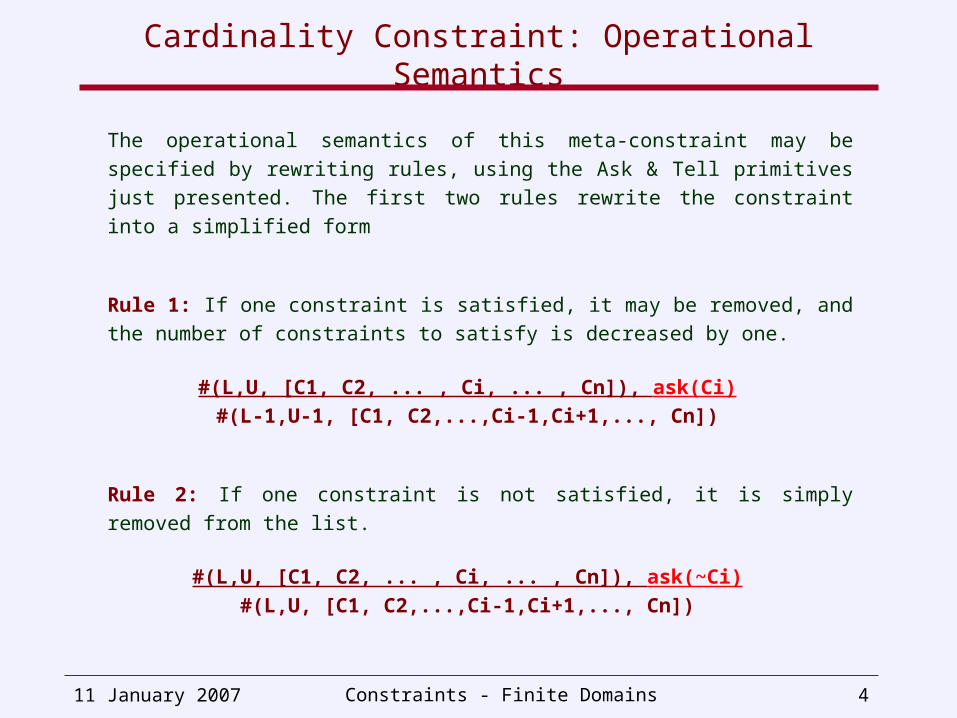
The operational semantics of this meta-constraint may be specified by
rewriting rules, using the Ask & Tell primitives just presented. The first two
rules rewrite the constraint into a simplified form
Rule 1: If one constraint is satisfied, it may be removed, and the number of
constraints to satisfy is decreased by one.
#(L,U, [C1, C2, ... , Ci, ... , Cn]), ask(Ci)
#(L-1,U-1, [C1, C2,...,Ci-1,Ci+1,..., Cn])
Rule 2: If one constraint is not satisfied, it is simply removed from the list.
#(L,U, [C1, C2, ... , Ci, ... , Cn]), ask(~Ci)
#(L,U, [C1, C2,...,Ci-1,Ci+1,..., Cn])
11 January 2007 Constraints - Finite Domains 5
Cardinality Constraint: Operational Semantics
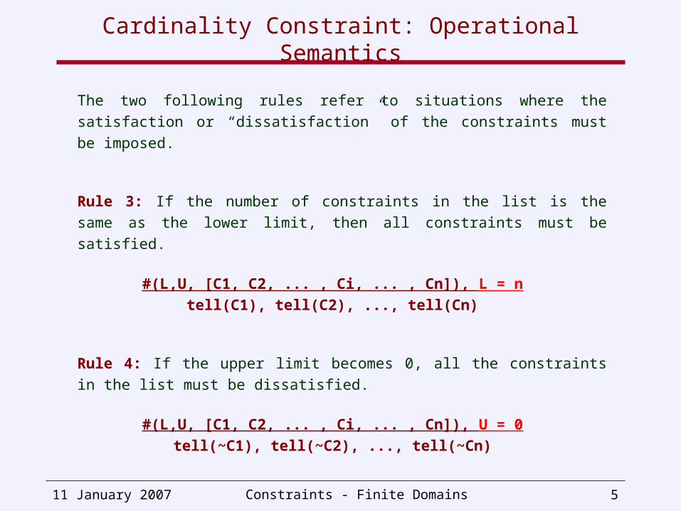
The two following rules refer to situations where the satisfaction or
“dissatisfaction” of the constraints must be imposed.
Rule 3: If the number of constraints in the list is the same as the lower limit,
then all constraints must be satisfied.
#(L,U, [C1, C2, ... , Ci, ... , Cn]), L = n
tell(C1), tell(C2), ..., tell(Cn)
Rule 4: If the upper limit becomes 0, all the constraints in the list must be
dissatisfied.
#(L,U, [C1, C2, ... , Ci, ... , Cn]), U = 0
tell(~C1), tell(~C2), ..., tell(~Cn)
11 January 2007 Constraints - Finite Domains 6
Cardinality Constraint: Operational Semantics
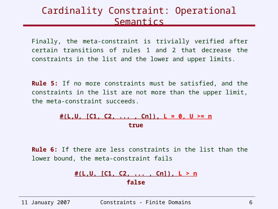
Finally, the meta-constraint is trivially verified after certain transitions of rules 1
and 2 that decrease the constraints in the list and the lower and upper limits.
Rule 5: If no more constraints must be satisfied, and the constraints in the list
are not more than the upper limit, the meta-constraint succeeds.
#(L,U, [C1, C2, ... , Cn]), L = 0, U >= n
true
Rule 6: If there are less constraints in the list than the lower bound, the meta-
constraint fails
#(L,U, [C1, C2, ... , Cn]), L > n
false
11 January 2007 Constraints - Finite Domains 7
Cardinality Constraint through Reified Constraints
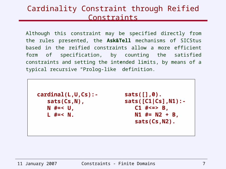
Although this constraint may be specified directly from the rules presented, the
Ask&Tell mechanisms of SICStus based in the reified constraints allow a more
efficient form of specification, by counting the satisfied constraints and setting
the intended limits, by means of a typical recursive “Prolog-like” definition.
cardinal(L,U,Cs):- sats(Cs,N), N #=< U, L #=< N.
sats([],0).sats([C1|Cs],N1):- C1 #<=> B, N1 #= N2 + B, sats(Cs,N2).
11 January 2007 Constraints - Finite Domains 8
Cardinality Constraint through Reified Constraints
The cardinality (meta-)constraint is genericaly applicable to combinations of
constraints requiring some form of counting.
Other combinations of constraints are possible to specify through the use of
reified constraints.
Among others, it is worth mentioning the case of conditional constraints, i.e.
those that should only be imposed if others are satisfied.
In scheduling, for example, it may be the case that only one of tasks T1 and T2
must finish before some time limit Z.
If this is task T2, then task T3 must start after some delay interval, I, starting
from the end of task T2.
11 January 2007 Constraints - Finite Domains 9
Conditional Constraints through Reification
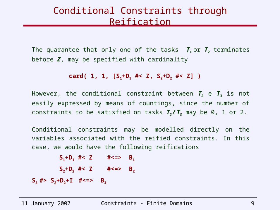
The guarantee that only one of the tasks T1 or T2 terminates before Z, may be
specified with cardinality
card( 1, 1, [S1+D1 #< Z, S2+D2 #< Z] )
However, the conditional constraint between T2 e T3 is not easily expressed by
means of countings, since the number of constraints to be satisfied on tasks
T2 / T3 may be 0, 1 or 2.
Conditional constraints may be modelled directly on the variables associated
with the reified constraints. In this case, we would have the following
reifications
S1+D1 #< Z #<=> B1
S2+D2 #< Z #<=> B2
S3 #> S2+D2+I #<=> B3
11 January 2007 Constraints - Finite Domains 10
Conditional Constraints through Reification
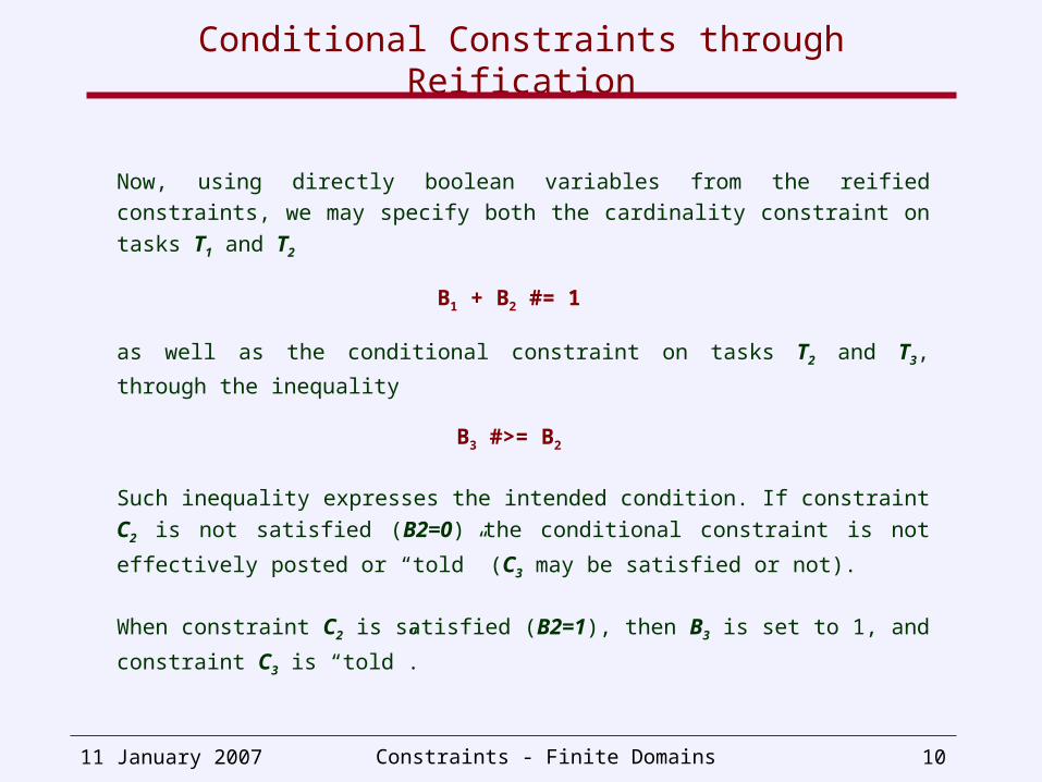
Now, using directly boolean variables from the reified constraints, we may
specify both the cardinality constraint on tasks T1 and T2
B1 + B2 #= 1
as well as the conditional constraint on tasks T2 and T3, through the inequality
B3 #>= B2
Such inequality expresses the intended condition. If constraint C2 is not
satisfied (B2=0) the conditional constraint is not effectively posted or “told” (C3
may be satisfied or not).
When constraint C2 is satisfied (B2=1), then B3 is set to 1, and constraint C3 is
“told”.
11 January 2007 Constraints - Finite Domains 11
Propositional Constraints
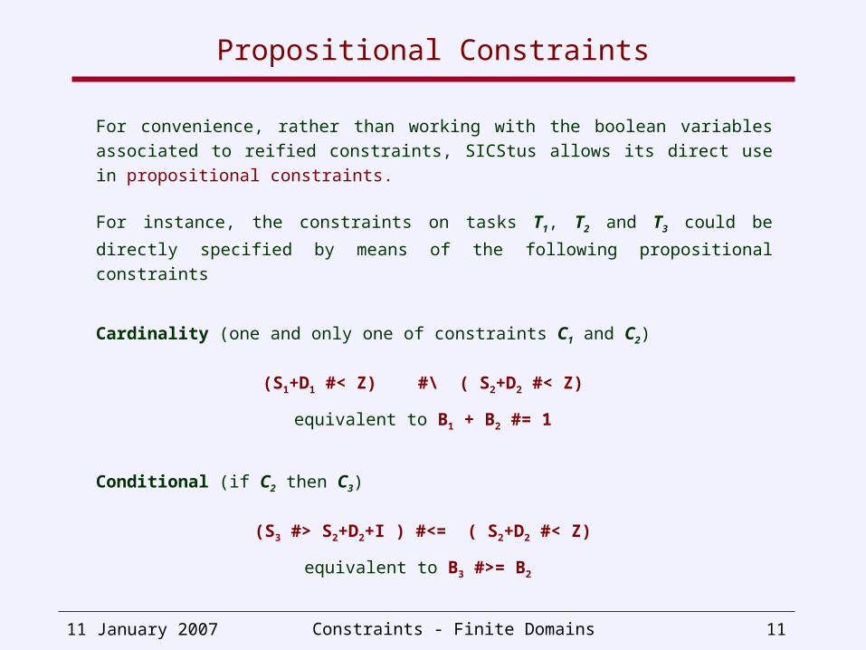
For convenience, rather than working with the boolean variables associated to
reified constraints, SICStus allows its direct use in propositional constraints.
For instance, the constraints on tasks T1, T2 and T3 could be directly specified
by means of the following propositional constraints
Cardinality (one and only one of constraints C1 and C2)
(S1+D1 #< Z) #\ ( S2+D2 #< Z)
equivalent to B1 + B2 #= 1
Conditional (if C2 then C3)
(S3 #> S2+D2+I ) #<= ( S2+D2 #< Z)
equivalent to B3 #>= B2
11 January 2007 Constraints - Finite Domains 12
Cardinality Constraint through Reified Constraints
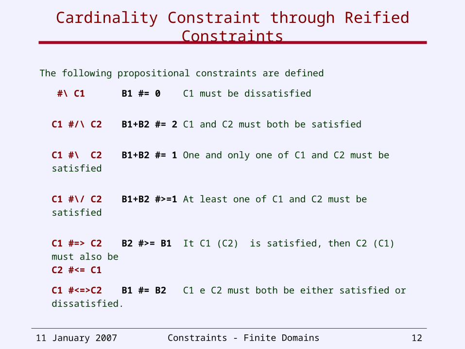
The following propositional constraints are defined
#\ C1 B1 #= 0 C1 must be dissatisfied
C1 #/\ C2 B1+B2 #= 2 C1 and C2 must both be satisfied
C1 #\ C2 B1+B2 #= 1 One and only one of C1 and C2 must be satisfied
C1 #\/ C2 B1+B2 #>=1 At least one of C1 and C2 must be satisfied
C1 #=> C2 B2 #>= B1 It C1 (C2) is satisfied, then C2 (C1) must also be
C2 #<= C1
C1 #<=>C2 B1 #= B2 C1 e C2 must both be either satisfied or
dissatisfied.
11 January 2007 Constraints - Finite Domains 13
Constructive Disjunction
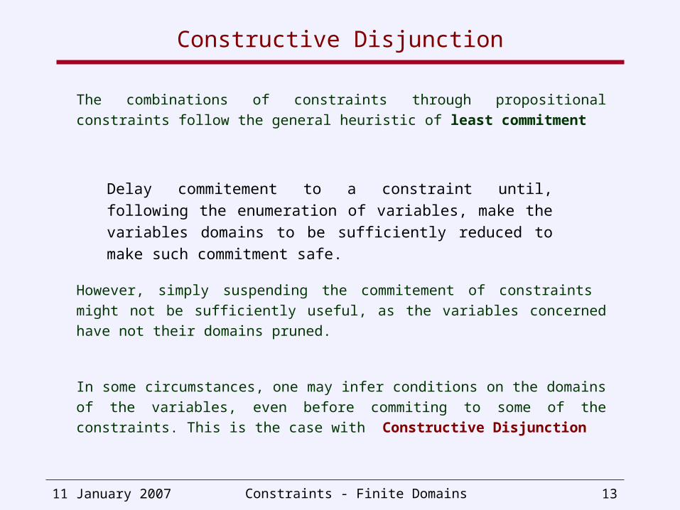
The combinations of constraints through propositional constraints follow the
general heuristic of least commitment
However, simply suspending the commitement of constraints might not be
sufficiently useful, as the variables concerned have not their domains pruned.
In some circumstances, one may infer conditions on the domains of the
variables, even before commiting to some of the constraints. This is the case
with Constructive Disjunction
Delay commitement to a constraint until, following the enumeration
of variables, make the variables domains to be sufficiently reduced
to make such commitment safe.
11 January 2007 Constraints - Finite Domains 14
Constructive Disjunction
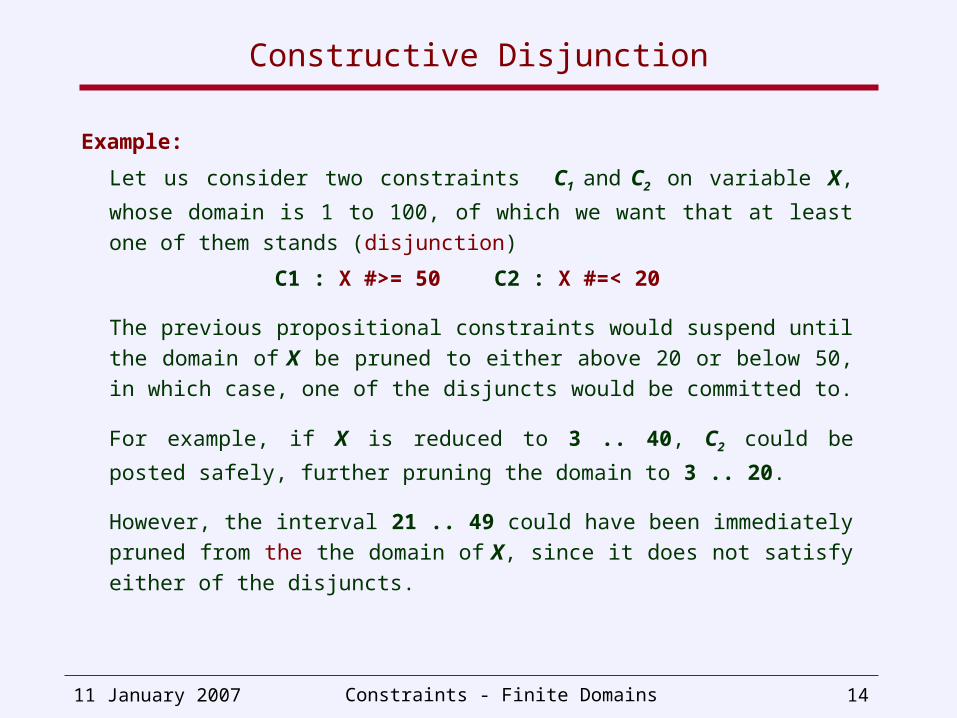
Example:
Let us consider two constraints C1 and C2 on variable X, whose domain is 1 to
100, of which we want that at least one of them stands (disjunction)
C1 : X #>= 50 C2 : X #=< 20
The previous propositional constraints would suspend until the domain of X be
pruned to either above 20 or below 50, in which case, one of the disjuncts
would be committed to.
For example, if X is reduced to 3 .. 40, C2 could be posted safely, further
pruning the domain to 3 .. 20.
However, the interval 21 .. 49 could have been immediately pruned from the
the domain of X, since it does not satisfy either of the disjuncts.
11 January 2007 Constraints - Finite Domains 15
Constructive Disjunction
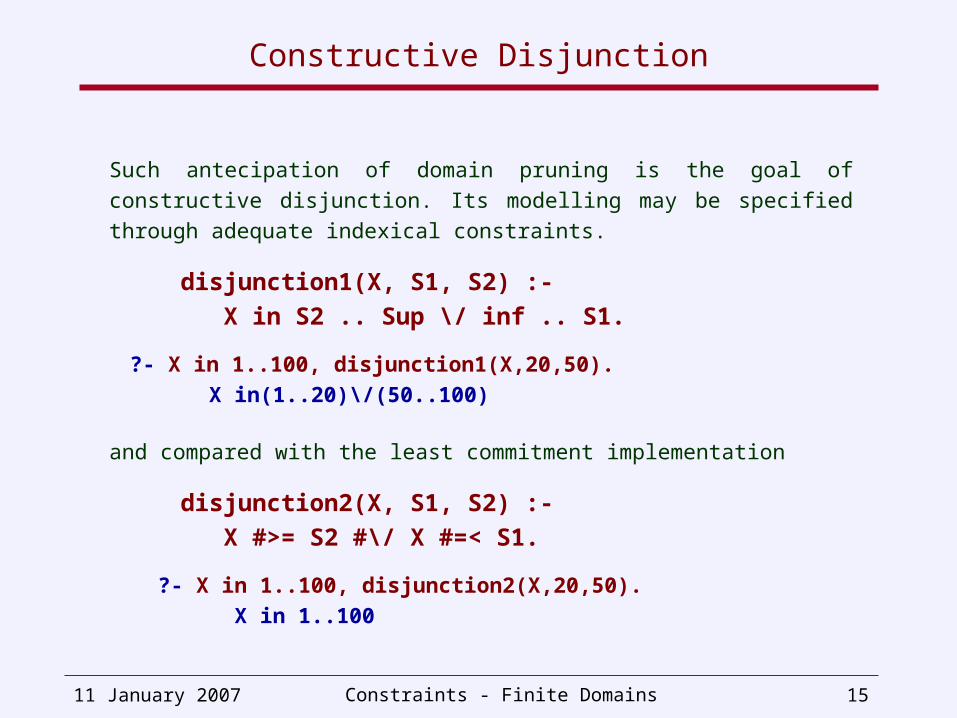
Such antecipation of domain pruning is the goal of constructive disjunction. Its
modelling may be specified through adequate indexical constraints.
disjunction1(X, S1, S2) :-
X in S2 .. Sup \/ inf .. S1.
?- X in 1..100, disjunction1(X,20,50).
X in(1..20)\/(50..100)
and compared with the least commitment implementation
disjunction2(X, S1, S2) :-
X #>= S2 #\/ X #=< S1.
?- X in 1..100, disjunction2(X,20,50).
X in 1..100
11 January 2007 Constraints - Finite Domains 16
Global Constraints: Generalised Arc Consistency
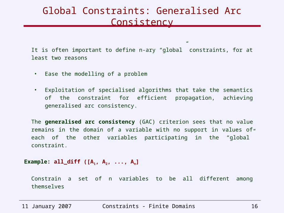
It is often important to define n-ary “global” constraints, for at least two reasons
• Ease the modelling of a problem
• Exploitation of specialised algorithms that take the semantics of the
constraint for efficient propagation, achieving generalised arc
consistency.
The generalised arc consistency (GAC) criterion sees that no value remains
in the domain of a variable with no support in values of each of the other
variables participating in the “global” constraint.
Example: all_diff ([A1, A2, ..., An]
Constrain a set of n variables to be all different among themselves
11 January 2007 Constraints - Finite Domains 17
Global Constraints: all_diff
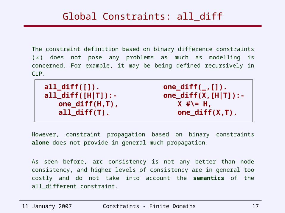
The constraint definition based on binary difference constraints () does not
pose any problems as much as modelling is concerned. For example, it may
be being defined recursively in CLP.
However, constraint propagation based on binary constraints alone does not
provide in general much propagation.
As seen before, arc consistency is not any better than node consistency, and
higher levels of consistency are in general too costly and do not take into
account the semantics of the all_different constraint.
one_diff(_,[]).one_diff(X,[H|T]):-
X #\= H, one_diff(X,T).
all_diff([]).all_diff([H|T]):-
one_diff(H,T),all_diff(T).
11 January 2007 Constraints - Finite Domains 18
Global Constraints: all_diff
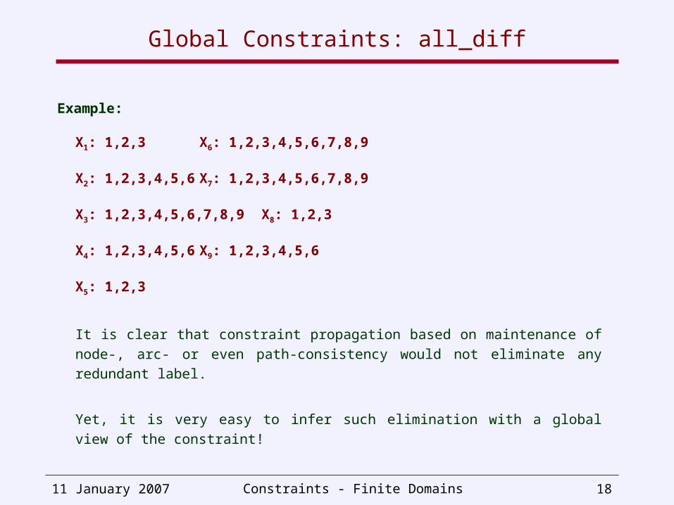
Example:
X1: 1,2,3 X6: 1,2,3,4,5,6,7,8,9
X2: 1,2,3,4,5,6 X7: 1,2,3,4,5,6,7,8,9
X3: 1,2,3,4,5,6,7,8,9 X8: 1,2,3
X4: 1,2,3,4,5,6 X9: 1,2,3,4,5,6
X5: 1,2,3
It is clear that constraint propagation based on maintenance of node-, arc- or
even path-consistency would not eliminate any redundant label.
Yet, it is very easy to infer such elimination with a global view of the constraint!
11 January 2007 Constraints - Finite Domains 19
Global Constraints: all_diff
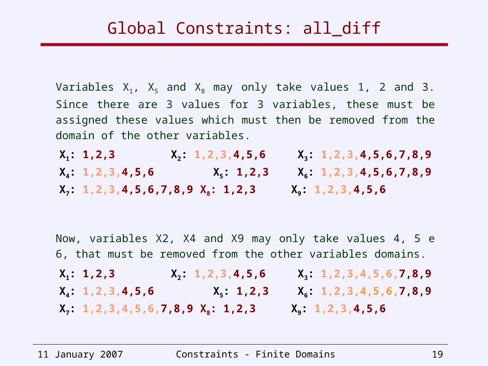
Variables X1, X5 and X8 may only take values 1, 2 and 3. Since there are 3
values for 3 variables, these must be assigned these values which must then
be removed from the domain of the other variables.
Now, variables X2, X4 and X9 may only take values 4, 5 e 6, that must be
removed from the other variables domains.
X1: 1,2,3 X2: 1,2,3,4,5,6 X3: 1,2,3,4,5,6,7,8,9
X4: 1,2,3,4,5,6 X5: 1,2,3 X6: 1,2,3,4,5,6,7,8,9
X7: 1,2,3,4,5,6,7,8,9 X8: 1,2,3 X9: 1,2,3,4,5,6
X1: 1,2,3 X2: 1,2,3,4,5,6 X3: 1,2,3,4,5,6,7,8,9
X4: 1,2,3,4,5,6 X5: 1,2,3 X6: 1,2,3,4,5,6,7,8,9
X7: 1,2,3,4,5,6,7,8,9 X8: 1,2,3 X9: 1,2,3,4,5,6
11 January 2007 Constraints - Finite Domains 20
Global Constraints: all_diff
In this case, these prunings could be obtained, by maintaining (strong) 4-
consistency.
For example, analysing variables X1, X2, X5 and X8, it would be “easy” to verify
that from the d4 potential assignments of values to them, no assignment would
include X2 = 1, X2 = 2, nor X2 = 3, thus leading to the prunning of X2 domain.
However, such maintenance is usually very expensive, computationally. For
each combination of 4 variables, d4 tuples whould be checked, with complexity
O(d4).
In fact, in some cases, n-strong consistency would be required, so its naïf
maintenance would be exponential on the number of variables, exactly what
one would like to avoid in search!
11 January 2007 Constraints - Finite Domains 21
Global Constraints: all_diff
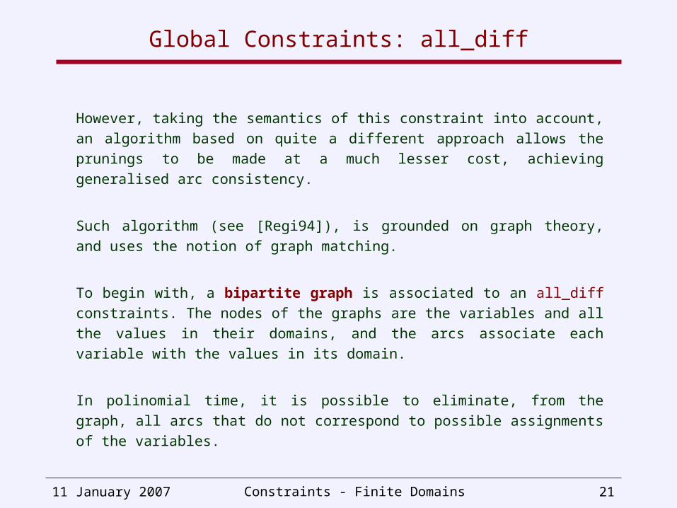
However, taking the semantics of this constraint into account, an algorithm
based on quite a different approach allows the prunings to be made at a much
lesser cost, achieving generalised arc consistency.
Such algorithm (see [Regi94]), is grounded on graph theory, and uses the
notion of graph matching.
To begin with, a bipartite graph is associated to an all_diff constraints. The
nodes of the graphs are the variables and all the values in their domains, and
the arcs associate each variable with the values in its domain.
In polinomial time, it is possible to eliminate, from the graph, all arcs that do not
correspond to possible assignments of the variables.
11 January 2007 Constraints - Finite Domains 22
Global Constraints: all_diff
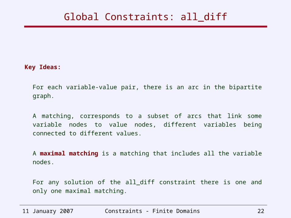
Key Ideas:
For each variable-value pair, there is an arc in the bipartite graph.
A matching, corresponds to a subset of arcs that link some variable nodes to
value nodes, different variables being connected to different values.
A maximal matching is a matching that includes all the variable nodes.
For any solution of the all_diff constraint there is one and only one maximal
matching.
11 January 2007 Constraints - Finite Domains 23
Global Constraints: all_diff
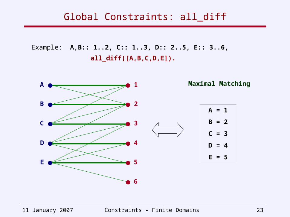
Example: A,B:: 1..2, C:: 1..3, D:: 2..5, E:: 3..6,
all_diff([A,B,C,D,E]).
A
B
C
D
E
1
2
3
4
5
6
A = 1
B = 2
C = 3
D = 4
E = 5
Maximal Matching
11 January 2007 Constraints - Finite Domains 24
Global Constraints: all_diff
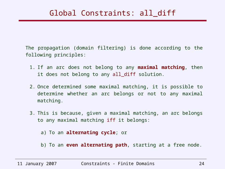
The propagation (domain filtering) is done according to the following principles:
1. If an arc does not belong to any maximal matching, then it does not
belong to any all_diff solution.
2. Once determined some maximal matching, it is possible to determine
whether an arc belongs or not to any maximal matching.
3. This is because, given a maximal matching, an arc belongs to any
maximal matching iff it belongs:
a) To an alternating cycle; or
b) To an even alternating path, starting at a free node.
11 January 2007 Constraints - Finite Domains 25
Global Constraints: all_diff
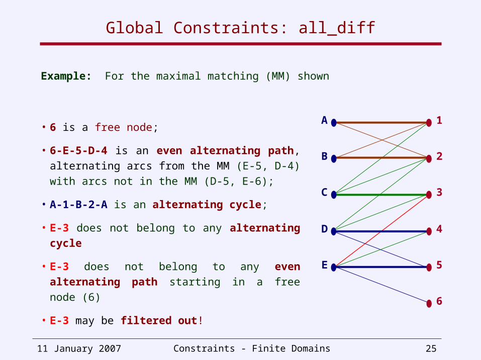
Example: For the maximal matching (MM) shown
• 6 is a free node;
• 6-E-5-D-4 is an even alternating path, alternating
arcs from the MM (E-5, D-4) with arcs not in the MM
(D-5, E-6);
• A-1-B-2-A is an alternating cycle;
• E-3 does not belong to any alternating cycle
• E-3 does not belong to any even alternating path
starting in a free node (6)
• E-3 may be filtered out!
A
B
C
D
E
1
2
3
4
5
6
11 January 2007 Constraints - Finite Domains 26
Global Constraints: all_diff
Compaction
Before this analysis, the graph may be “compacted”, aggregating, into a
single node, “equivalent nodes”, i.e. those belonging to alternating cycles.
Intuitively, for any solution involving these variables and values, a different
solution may be obtained by permutation of the corresponding
assignments.
Hence, the filtering analysis may be made based on any of these
solutions, hence the set of nodes can be grouped in a single one.
11 January 2007 Constraints - Finite Domains 27
Global Constraints: all_diff
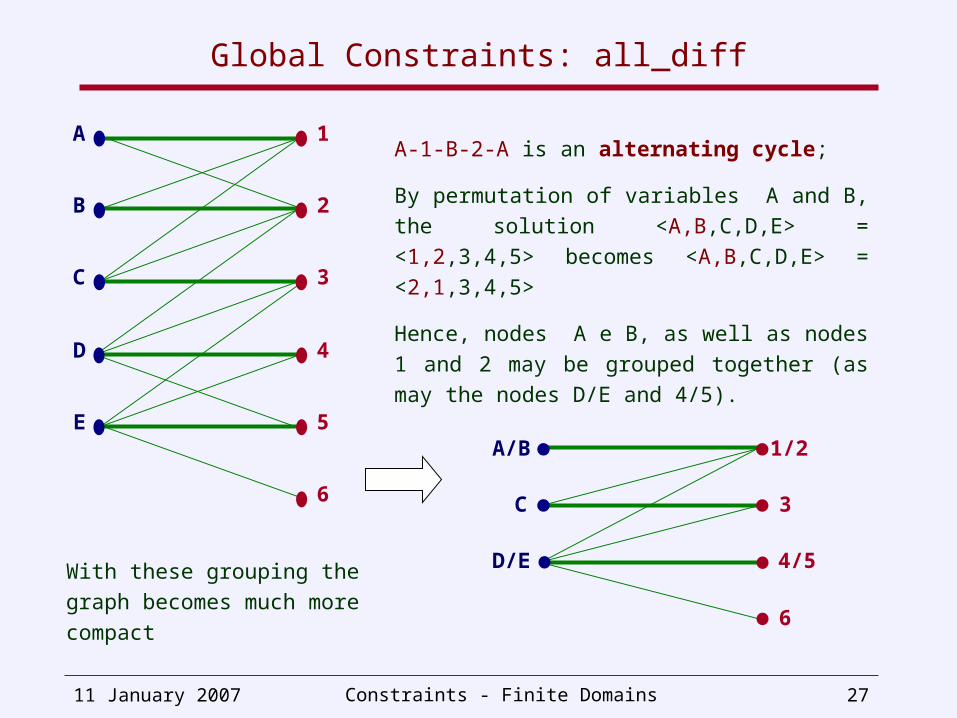
A-1-B-2-A is an alternating cycle;
By permutation of variables A and B, the solution
<A,B,C,D,E> = <1,2,3,4,5> becomes <A,B,C,D,E>
= <2,1,3,4,5>
Hence, nodes A e B, as well as nodes 1 and 2
may be grouped together (as may the nodes D/E
and 4/5).
A/B
C
4/5
3
6
D/E
1/2
A
B
C
D
E
1
2
3
4
5
6
With these grouping the graph
becomes much more compact
11 January 2007 Constraints - Finite Domains 28
Global Constraints: all_diff
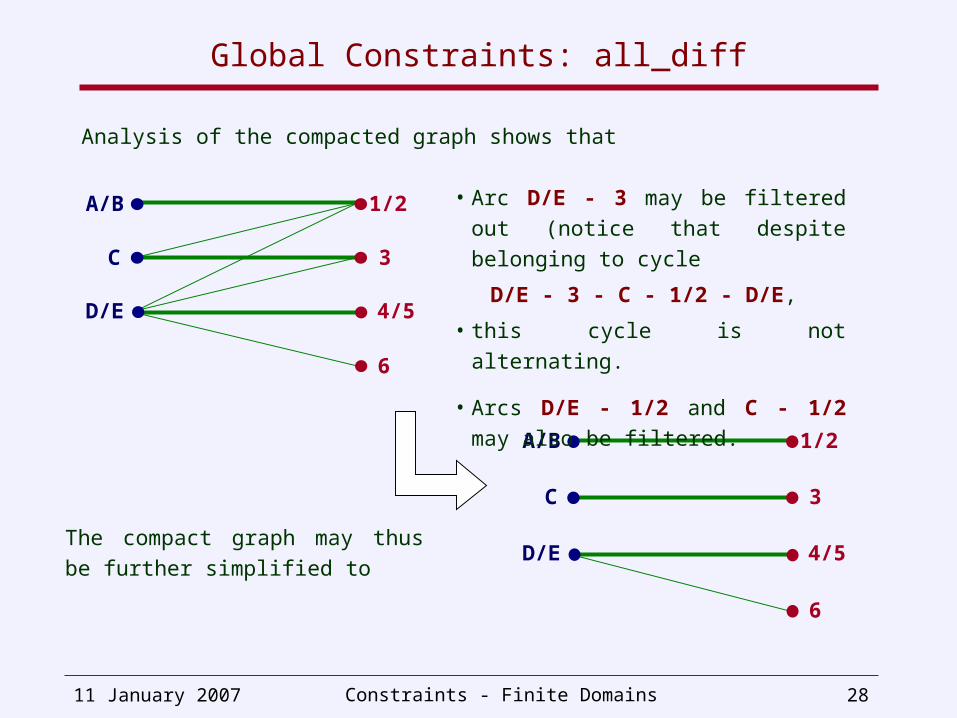
Analysis of the compacted graph shows that
A/B
C
4/5
3
6
D/E
1/2
A/B
C
4/5
3
6
D/E
1/2
• Arc D/E - 3 may be filtered out (notice
that despite belonging to cycle
D/E - 3 - C - 1/2 - D/E,
• this cycle is not alternating.
• Arcs D/E - 1/2 and C - 1/2 may also be
filtered.
The compact graph may thus be
further simplified to
11 January 2007 Constraints - Finite Domains 29
Global Constraints: all_diff
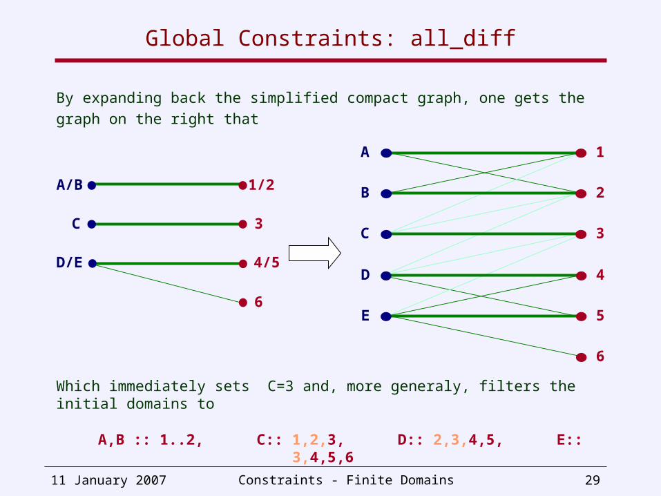
By expanding back the simplified compact graph, one gets the graph on the right
that
A/B
C
4/5
3
6
D/E
1/2
Which immediately sets C=3 and, more generaly, filters the initial domains to
A,B :: 1..2, C:: 1,2,3, D:: 2,3,4,5, E:: 3,4,5,6
A
B
C
D
E
1
2
3
4
5
6
11 January 2007 Constraints - Finite Domains 30
Global Constraints: all_diff
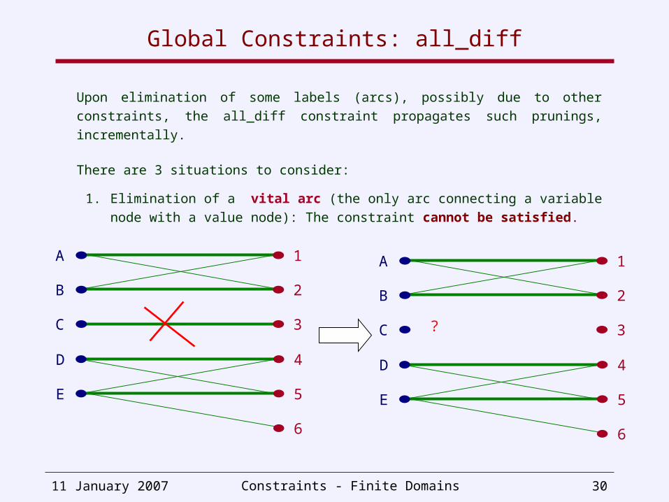
Upon elimination of some labels (arcs), possibly due to other constraints, the
all_diff constraint propagates such prunings, incrementally.
There are 3 situations to consider:
1. Elimination of a vital arc (the only arc connecting a variable node with a
value node): The constraint cannot be satisfied.
A
B
C
D
E
1
2
3
4
5
6
A
B
C
D
E
1
2
3
4
5
6
?
11 January 2007 Constraints - Finite Domains 31
Global Constraints: all_diff
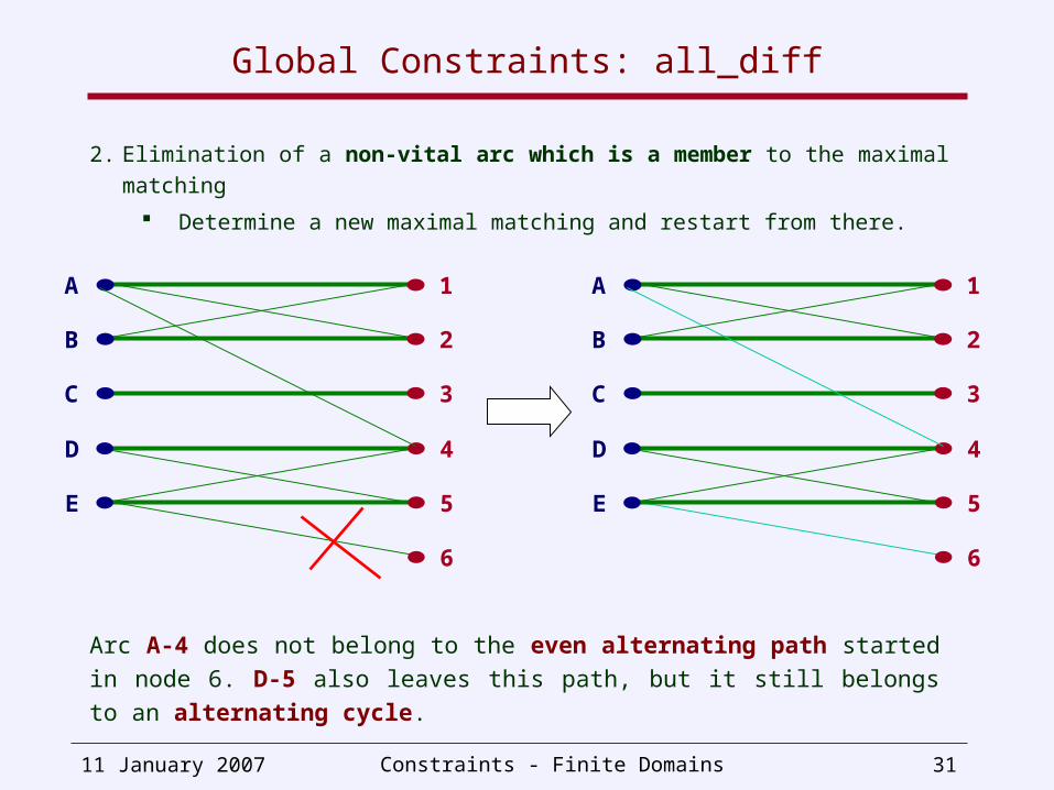
2. Elimination of a non-vital arc which is a member to the maximal matching
Determine a new maximal matching and restart from there.
A
B
C
D
E
1
2
3
4
5
6
A
B
C
D
E
1
2
3
4
5
6
Arc A-4 does not belong to the even alternating path started in node 6. D-5 also
leaves this path, but it still belongs to an alternating cycle.
11 January 2007 Constraints - Finite Domains 32
Global Constraints: all_diff
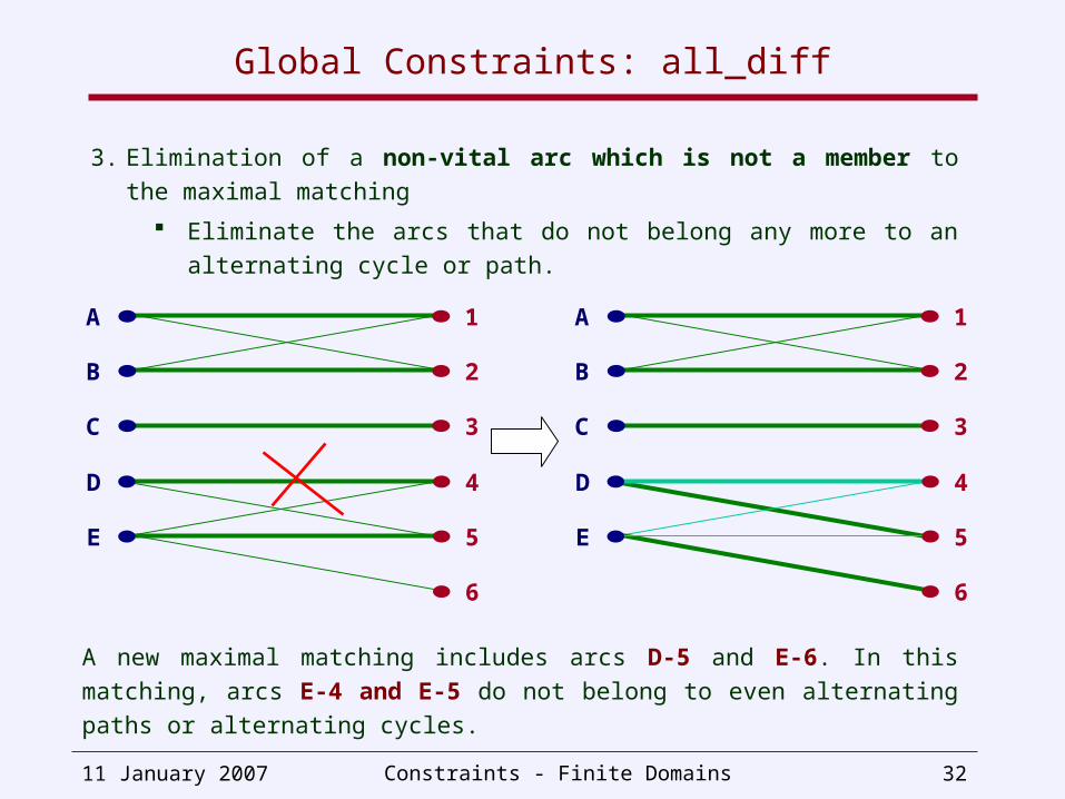
3. Elimination of a non-vital arc which is not a member to the maximal
matching
Eliminate the arcs that do not belong any more to an alternating cycle or
path.
A new maximal matching includes arcs D-5 and E-6. In this matching, arcs E-4 and
E-5 do not belong to even alternating paths or alternating cycles.
A
B
C
D
E
1
2
3
4
5
6
A
B
C
D
E
1
2
3
4
5
6
11 January 2007 Constraints - Finite Domains 33
Global Constraints: all_diff
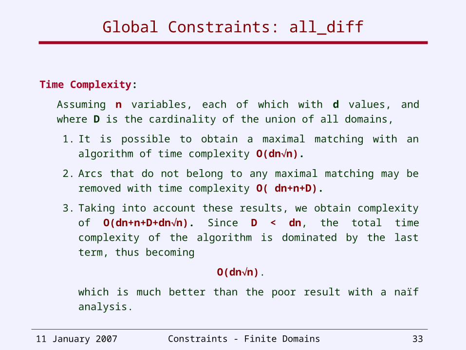
Time Complexity:
Assuming n variables, each of which with d values, and where D is the
cardinality of the union of all domains,
1. It is possible to obtain a maximal matching with an algorithm of time
complexity O(dnn).
2. Arcs that do not belong to any maximal matching may be removed with
time complexity O( dn+n+D).
3. Taking into account these results, we obtain complexity of
O(dn+n+D+dnn). Since D < dn, the total time complexity of the
algorithm is dominated by the last term, thus becoming
O(dnn).
which is much better than the poor result with a naïf analysis.
11 January 2007 Constraints - Finite Domains 34
Global Constraints: all_diff
Availability:
1. The all_diff constraint first appeared in the CHIP system (algorithm?).
2. The described implementation is incorporated into the ILOG system, and
avalable as primitive IlcAllDiff.
3. This algorithm is also implemented in SICStus, through buit-in constraint
all_distinct/1.
4. Other versions of the constraint, namely all _different/2, are also available,
possibly using a faster algorithm but with less pruning, where the 2nd argument
controls the available pruning options.
11 January 2007 Constraints - Finite Domains 35
Global Constraints: all_diff
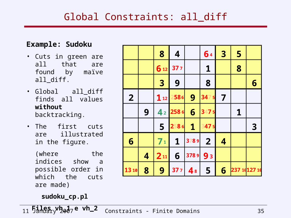
Example: Sudoku
• Cuts in green are all that are found by maïve all_diff.
• Global all_diff finds all values without backtracking.
• The first cuts are illustrated in the figure.
(where the indices show a possible order in which the cuts are made)
sudoku_cp.pl
Files vh_1 e vh_2
8 4 6 4 3 5
6 12 37 7 1 8
3 9 8 6
2 1 12 258 6 9 347 5 7
9 4 2 258 6 6 347 5 1
5 258 6 1 347 5 3
6 7 1 1 378 9 2 4
4 2 11 6 378 9 9 3
13 10 8 9 37 7 4 8 5 6 237 10127 10
11 January 2007 Constraints - Finite Domains 36
Global Constraints: circuit
The previous global constraints may be regarded as imposing a certain
“permutation” on the variables.
In many problems, such permutation is not a sufficient constraint. It is
necessary to impose a certain “ordering” of the variables.
A typical situation occurs when there is a sequencing of tasks, with
precedences between tasks, possibly with non-adjacency constraints between
some of them.
In these situations, in addition to the permutation of the variables, one must
ensure that the ordering of the tasks makes a single cycle, i.e. there must be
no sub-cycles.
11 January 2007 Constraints - Finite Domains 37
Global Constraints: circuit
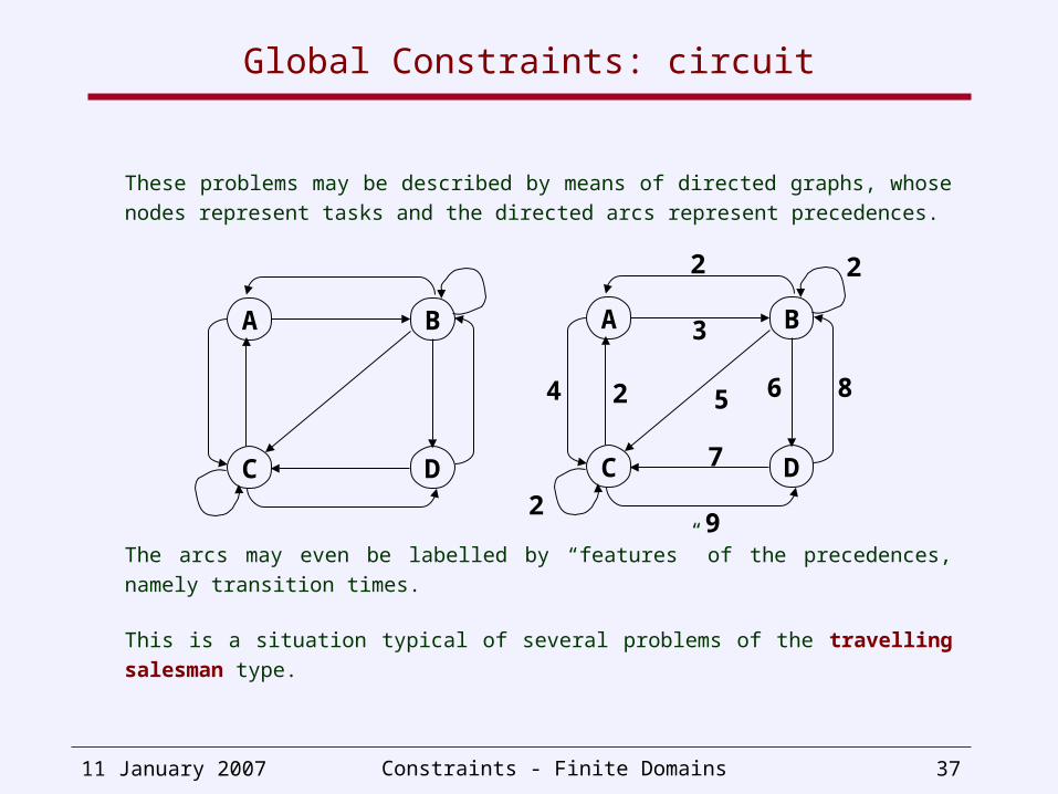
These problems may be described by means of directed graphs, whose nodes
represent tasks and the directed arcs represent precedences.
The arcs may even be labelled by “features” of the precedences, namely
transition times.
This is a situation typical of several problems of the travelling salesman type.
A B
C D
A B
C D
2
3
4 5 6
9
8
7
2
2
2
11 January 2007 Constraints - Finite Domains 38
Global Constraints: circuit
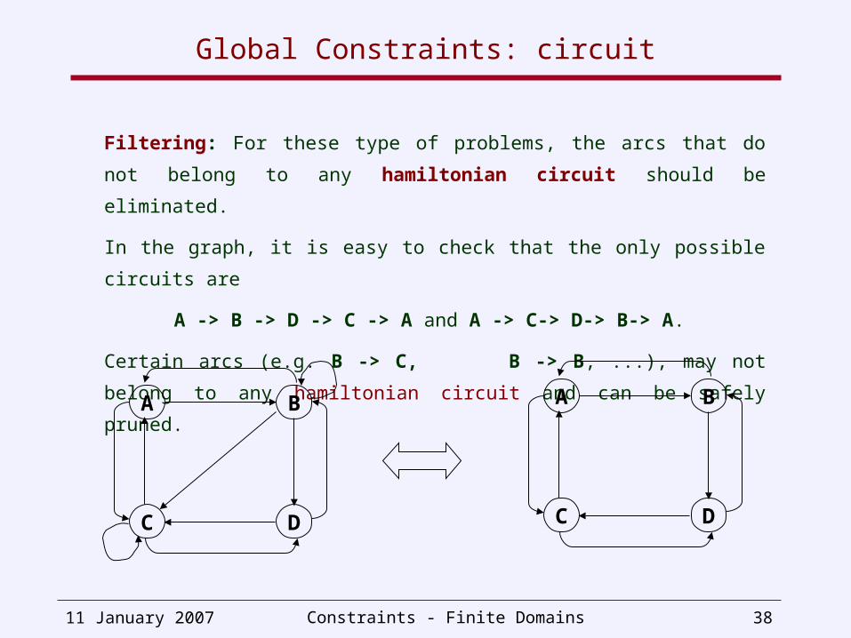
Filtering: For these type of problems, the arcs that do not belong to any
hamiltonian circuit should be eliminated.
In the graph, it is easy to check that the only possible circuits are
A -> B -> D -> C -> A and A -> C-> D-> B-> A.
Certain arcs (e.g. B -> C, B -> B, ...), may not belong to any hamiltonian
circuit and can be safely pruned.
A B
C D
A B
C D
11 January 2007 Constraints - Finite Domains 39
Global Constraints: circuit
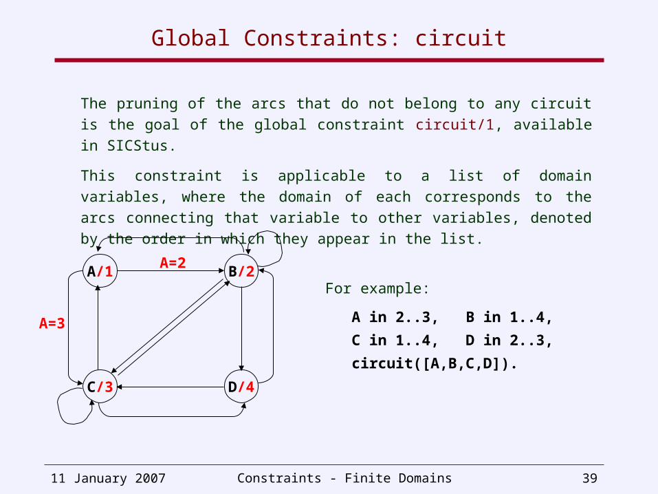
The pruning of the arcs that do not belong to any circuit is the goal of the
global constraint circuit/1, available in SICStus.
This constraint is applicable to a list of domain variables, where the domain of
each corresponds to the arcs connecting that variable to other variables,
denoted by the order in which they appear in the list.
For example:
A in 2..3, B in 1..4,
C in 1..4, D in 2..3,
circuit([A,B,C,D]).
A/1 B/2
C/3 D/4
A=2
A=3
11 January 2007 Constraints - Finite Domains 40
Global Constraints: circuit
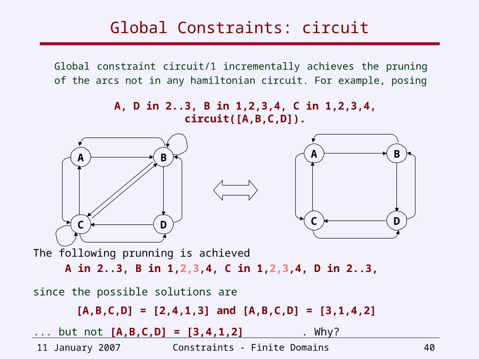
Global constraint circuit/1 incrementally achieves the pruning of the arcs not in
any hamiltonian circuit. For example, posing
A, D in 2..3, B in 1,2,3,4, C in 1,2,3,4,circuit([A,B,C,D]).
The following prunning is achieved
A in 2..3, B in 1,2,3,4, C in 1,2,3,4, D in 2..3,
since the possible solutions are
[A,B,C,D] = [2,4,1,3] and [A,B,C,D] = [3,1,4,2]
... but not [A,B,C,D] = [3,4,1,2] . Why?
A B
C D
A B
C D
11 January 2007 Constraints - Finite Domains 41
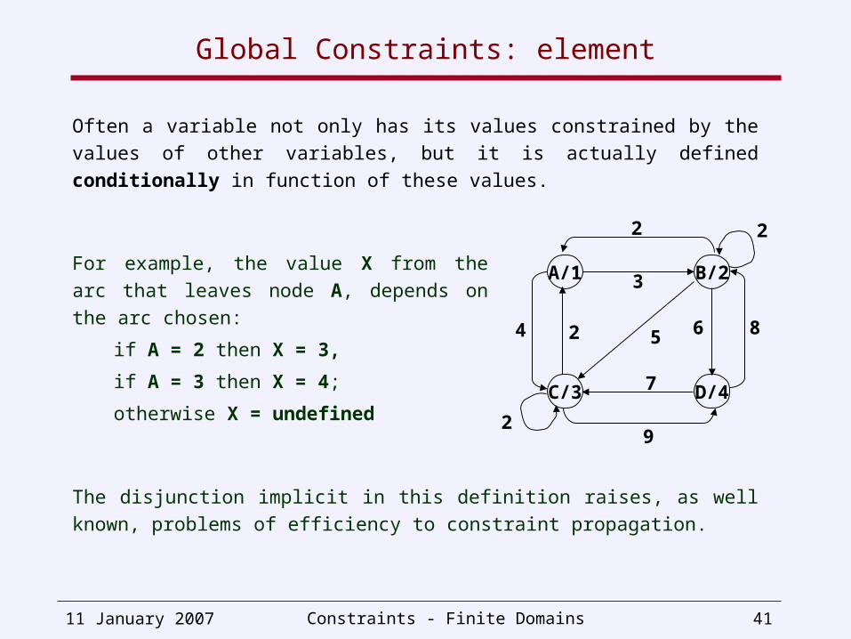
Global Constraints: element
For example, the value X from the arc that leaves
node A, depends on the arc chosen:
if A = 2 then X = 3,
if A = 3 then X = 4;
otherwise X = undefined
A/1 B/2
C/3 D/4
2
3
4 5 6
9
8
7
2
2
2
The disjunction implicit in this definition raises, as well known, problems of
efficiency to constraint propagation.
Often a variable not only has its values constrained by the values of other
variables, but it is actually defined conditionally in function of these values.
11 January 2007 Constraints - Finite Domains 42
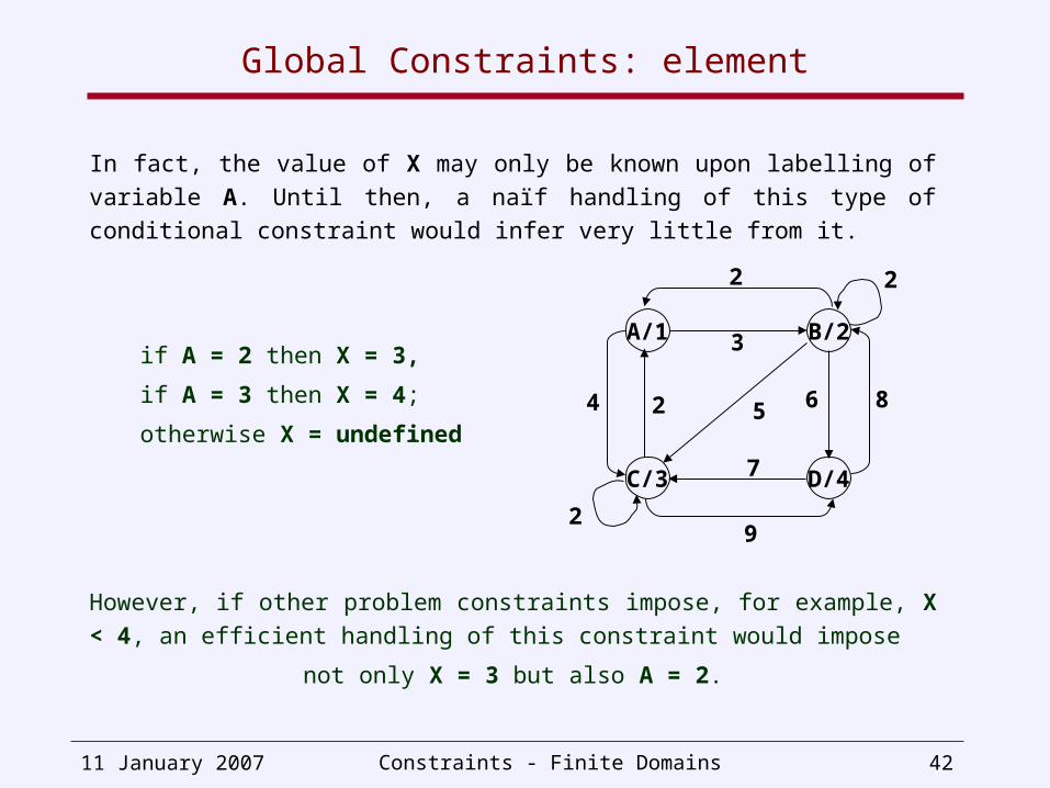
Global Constraints: element
In fact, the value of X may only be known upon labelling of variable A. Until then,
a naïf handling of this type of conditional constraint would infer very little from it.
A/1 B/2
C/3 D/4
2
3
4 5 6
9
8
7
2
2
2
However, if other problem constraints impose, for example, X < 4, an efficient
handling of this constraint would impose
not only X = 3 but also A = 2.
if A = 2 then X = 3,
if A = 3 then X = 4;
otherwise X = undefined
11 January 2007 Constraints - Finite Domains 43
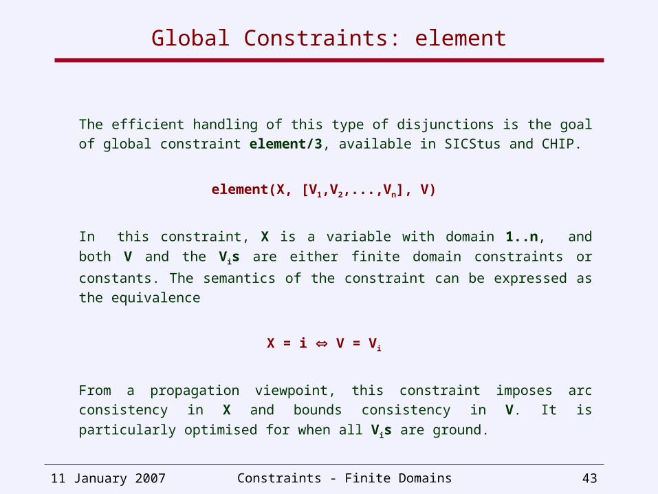
Global Constraints: element
The efficient handling of this type of disjunctions is the goal of global constraint
element/3, available in SICStus and CHIP.
element(X, [V1,V2,...,Vn], V)
In this constraint, X is a variable with domain 1..n, and both V and the Vis are
either finite domain constraints or constants. The semantics of the constraint
can be expressed as the equivalence
X = i V = Vi
From a propagation viewpoint, this constraint imposes arc consistency in X
and bounds consistency in V. It is particularly optimised for when all Vis are
ground.
11 January 2007 Constraints - Finite Domains 44
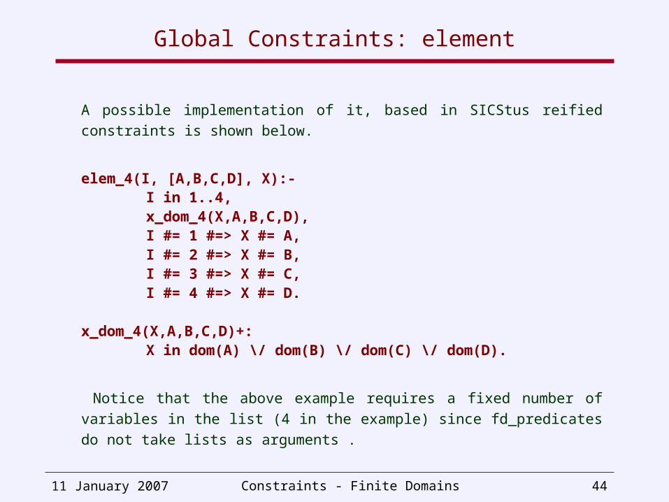
Global Constraints: element
A possible implementation of it, based in SICStus reified constraints is shown
below.
elem_4(I, [A,B,C,D], X):- I in 1..4, x_dom_4(X,A,B,C,D), I #= 1 #=> X #= A, I #= 2 #=> X #= B, I #= 3 #=> X #= C, I #= 4 #=> X #= D.
x_dom_4(X,A,B,C,D)+: X in dom(A) \/ dom(B) \/ dom(C) \/ dom(D).
Notice that the above example requires a fixed number of variables in the list
(4 in the example) since fd_predicates do not take lists as arguments .
11 January 2007 Constraints - Finite Domains 45
Global Constraints: element
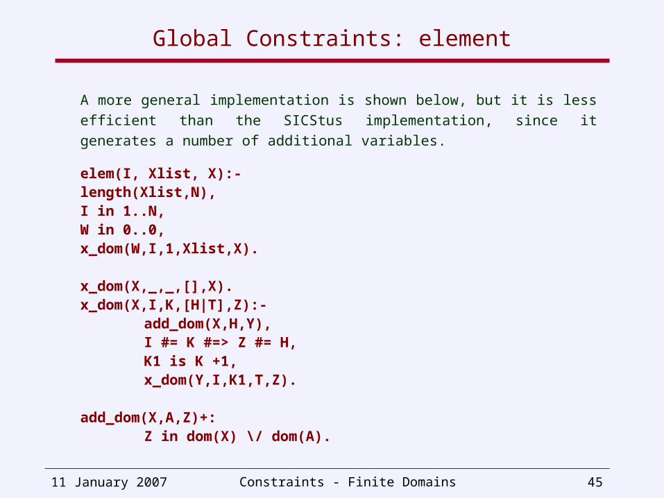
A more general implementation is shown below, but it is less efficient than the
SICStus implementation, since it generates a number of additional variables.
elem(I, Xlist, X):- length(Xlist,N), I in 1..N, W in 0..0, x_dom(W,I,1,Xlist,X).
x_dom(X,_,_,[],X).x_dom(X,I,K,[H|T],Z):-
add_dom(X,H,Y), I #= K #=> Z #= H, K1 is K +1, x_dom(Y,I,K1,T,Z).
add_dom(X,A,Z)+: Z in dom(X) \/ dom(A).
11 January 2007 Constraints - Finite Domains 46
Global Constraints: element
The previous global constraints may be regarded as imposing a certain
“permutation” on the variables.
In many problems, such permutation is not a sufficient constraint. It is
necessary to impose a certain “ordering” of the variables.
A typical situation occurs when there is a sequencing of tasks, with
precedences between tasks, possibly with non-adjacency constraints between
some of them.
In these situations, in addition to the permutation of the variables, one must
ensure that the ordering of the tasks makes a single cycle, i.e. there must be
no sub-cycles.
11 January 2007 Constraints - Finite Domains 47
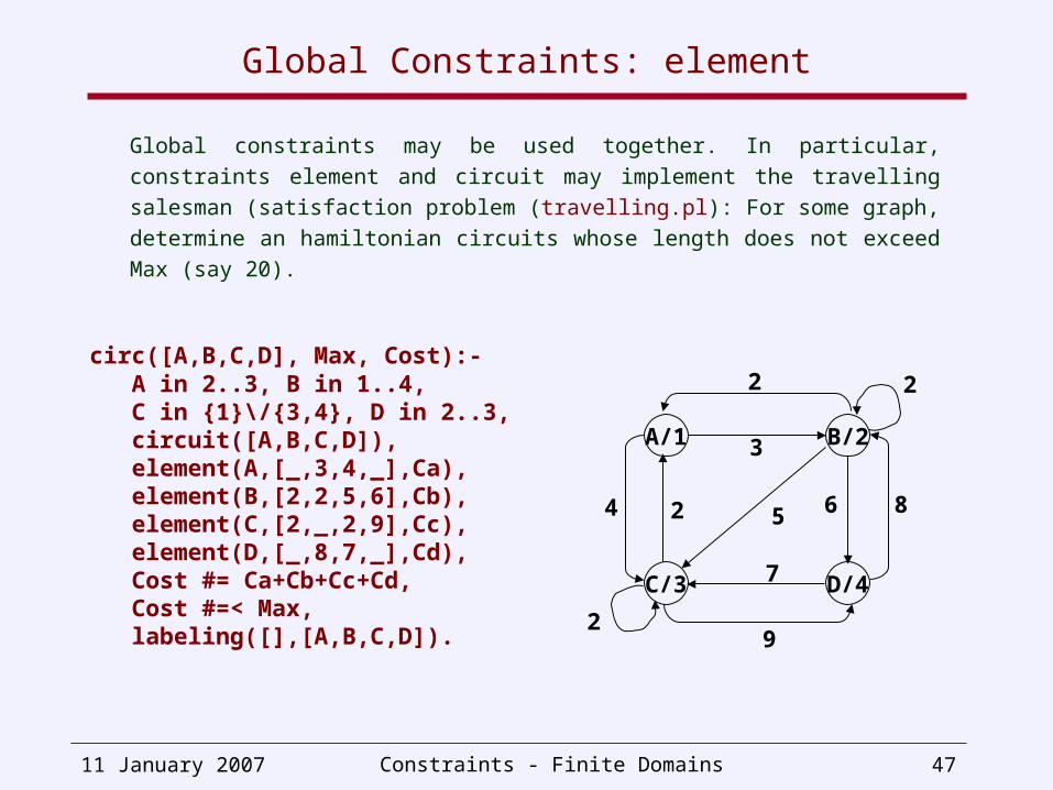
Global Constraints: element
Global constraints may be used together. In particular, constraints element
and circuit may implement the travelling salesman (satisfaction problem
(travelling.pl): For some graph, determine an hamiltonian circuits whose
length does not exceed Max (say 20).
circ([A,B,C,D], Max, Cost):- A in 2..3, B in 1..4, C in {1}\/{3,4}, D in 2..3, circuit([A,B,C,D]), element(A,[_,3,4,_],Ca), element(B,[2,2,5,6],Cb), element(C,[2,_,2,9],Cc), element(D,[_,8,7,_],Cd), Cost #= Ca+Cb+Cc+Cd, Cost #=< Max, labeling([],[A,B,C,D]).
A/1 B/2
C/3 D/4
2
3
4 5 6
9
8
7
2
2
2
11 January 2007 Constraints - Finite Domains 48
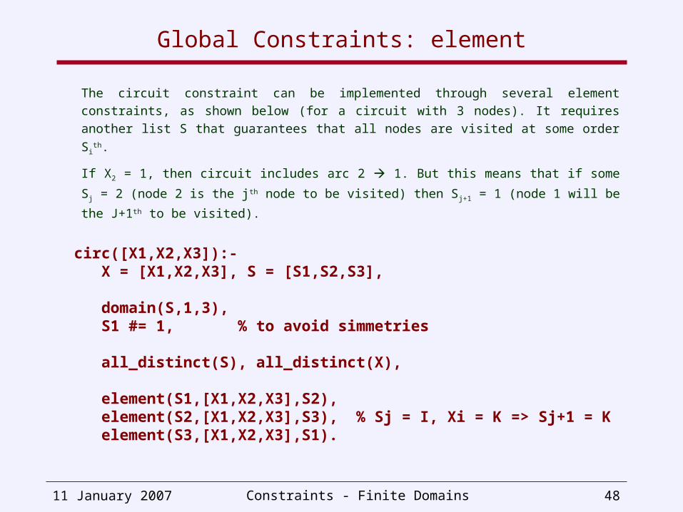
Global Constraints: element
The circuit constraint can be implemented through several element constraints, as
shown below (for a circuit with 3 nodes). It requires another list S that guarantees
that all nodes are visited at some order Sith.
If X2 = 1, then circuit includes arc 2 1. But this means that if some Sj = 2 (node
2 is the jth node to be visited) then Sj+1 = 1 (node 1 will be the J+1th to be visited).
circ([X1,X2,X3]):- X = [X1,X2,X3], S = [S1,S2,S3], domain(S,1,3), S1 #= 1, % to avoid simmetries
all_distinct(S), all_distinct(X),
element(S1,[X1,X2,X3],S2), element(S2,[X1,X2,X3],S3), % Sj = I, Xi = K => Sj+1 = K element(S3,[X1,X2,X3],S1).
11 January 2007 Constraints - Finite Domains 49
Global Constraints: cycle
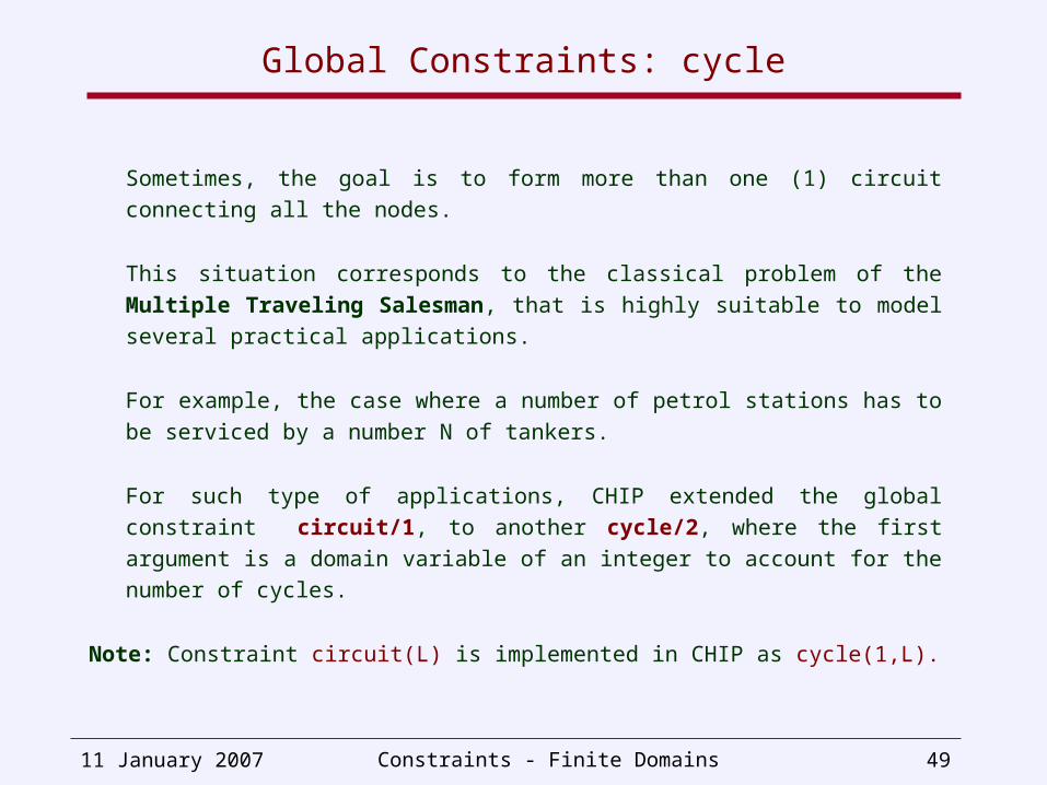
Sometimes, the goal is to form more than one (1) circuit connecting all the
nodes.
This situation corresponds to the classical problem of the Multiple Traveling
Salesman, that is highly suitable to model several practical applications.
For example, the case where a number of petrol stations has to be serviced by
a number N of tankers.
For such type of applications, CHIP extended the global constraint circuit/1,
to another cycle/2, where the first argument is a domain variable of an integer
to account for the number of cycles.
Note: Constraint circuit(L) is implemented in CHIP as cycle(1,L).
11 January 2007 Constraints - Finite Domains 50
Global Constraints: cycle
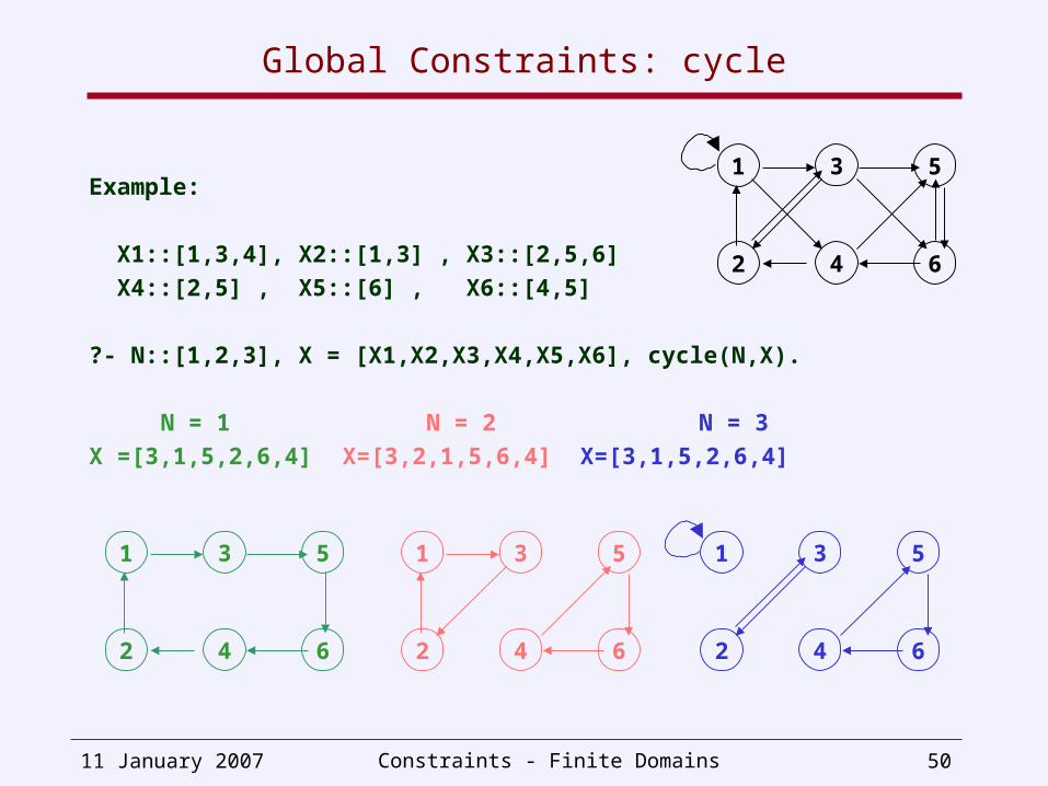
Example:
X1::[1,3,4], X2::[1,3] , X3::[2,5,6]
X4::[2,5] , X5::[6] , X6::[4,5]
?- N::[1,2,3], X = [X1,X2,X3,X4,X5,X6], cycle(N,X).
N = 1 N = 2 N = 3
X =[3,1,5,2,6,4] X=[3,2,1,5,6,4] X=[3,1,5,2,6,4]
2 4 6
1 3 5
2 4 6
1 3 5
2 4 6
1 3 5
2 4 6
1 3 5


![Constraint Logic Programming - MathUniPDfrossi/gulp.pdf · solvers added to a LP language becomes almost unlimited (e.g., [110]). 2.1 Finite Domains A popular class of constraints](https://img.dokumen.tips/doc/110x75/5f43502ab529c74c64766ec3/constraint-logic-programming-mathunipd-frossigulppdf-solvers-added-to-a-lp.jpg)