Embed Size (px)
Citation preview

Chair for Energy Trading & FinanceProf. Dr. Rüdiger Kiesel
10th Winter School– Energy MarketsLecture 3
Risk Premia in Energy Markets II
Professor Dr. Rüdiger Kiesel
Faculty of EconomicsChair of Energy Trading & Finance
Centre of Mathematics for Applications,University of Oslo
25. January 2011
An Equilibrium Approach Information Approach 1 / 72

Chair for Energy Trading & FinanceProf. Dr. Rüdiger Kiesel
1 An Equilibrium ApproachRepresentative Agents, Forward Dynamics and Market PowerMarket Price of Risk and Market Risk PremiumExamples and Empirical Evidence
2 Information Approach
An Equilibrium Approach Information Approach 2 / 72

Chair for Energy Trading & FinanceProf. Dr. Rüdiger Kiesel
Agenda
1 An Equilibrium ApproachRepresentative Agents, Forward Dynamics and Market PowerMarket Price of Risk and Market Risk PremiumExamples and Empirical Evidence
2 Information Approach
An Equilibrium Approach Information Approach 3 / 72Representative Agents, Forward Dynamics and Market Power Market Price of Risk and Market Risk Premium Examples and Empirical Evidence

Chair for Energy Trading & FinanceProf. Dr. Rüdiger Kiesel
Market Risk Premium – Players
The main motivation for players to engage in forward contracts isthat of risk diversification.Producers have made large investments with the aim of recoupingthem over a long period of time as well as making a return on them.Retailers (which might be intermediaries and/or use the commodityin their production process) also have an incentive to hedge theirpositions in the market by contracting forwards that help diversifytheir risks.
An Equilibrium Approach Information Approach 4 / 72Representative Agents, Forward Dynamics and Market Power Market Price of Risk and Market Risk Premium Examples and Empirical Evidence

Chair for Energy Trading & FinanceProf. Dr. Rüdiger Kiesel
Market Risk Premium – Qualitative
Exposure to the market will differ both between producers andretailers as well as within their own group.For example, a large producer will generally be exposed to marketuncertainty for a longer period of time, perhaps determined by theremaining life of the assets, whilst retailers will tend to makedecisions based on a shorter time scale.So the need for risk-diversification has a temporal dimension.
An Equilibrium Approach Information Approach 5 / 72Representative Agents, Forward Dynamics and Market Power Market Price of Risk and Market Risk Premium Examples and Empirical Evidence

Chair for Energy Trading & FinanceProf. Dr. Rüdiger Kiesel
Market Risk Premium
These differences in the desire to hedge positions are employedto explain the market risk premium and its sign.Retailers are less incentivized to contract commodity forwardsthe further out we look into the market.In contrast, on the producers’ side the need to hedge in thelong-term does not fade away as quickly.
An Equilibrium Approach Information Approach 6 / 72Representative Agents, Forward Dynamics and Market Power Market Price of Risk and Market Risk Premium Examples and Empirical Evidence

Chair for Energy Trading & FinanceProf. Dr. Rüdiger Kiesel
Market Risk Premium
We associate situations where π(t,T ) > 0 with the fact thatretailers’ desire to cover their positions ‘outweighs’ those of theproducers, resulting in a positive market risk premium.The mirror image is therefore one where the producers’ desireto hedge their positions outweighs that of the retailersresulting in a negative market risk premium.
An Equilibrium Approach Information Approach 7 / 72Representative Agents, Forward Dynamics and Market Power Market Price of Risk and Market Risk Premium Examples and Empirical Evidence
Chair for Energy Trading & FinanceProf. Dr. Rüdiger Kiesel
Representative Agents
We describe producers’ and retailers’ preferences via the utilityfunction of two representative agents.Agents must decide how to manage their exposure to the spotand forward markets for every future date T .A key question for the producer is how much of his futureproduction, which cannot be predicted with total certainty, willhe wish to sell on the forward market or, when the time comes,sell it on the spot market.Similarly, the retailer must decide how much of her futureneeds, which cannot be predicted with full certainty either, willbe acquired via the forward markets and how much on thespot.
An Equilibrium Approach Information Approach 8 / 72Representative Agents, Forward Dynamics and Market Power Market Price of Risk and Market Risk Premium Examples and Empirical Evidence
Chair for Energy Trading & FinanceProf. Dr. Rüdiger Kiesel
Representative Agents
We approach this financial decision and equilibrium price formationin two steps.
First, we determine the forward price that makes the agentsindifferent between the forward and spot market.Second, we discuss how the relative willingness of producersand retailers to hedge their exposures determines marketclearing prices.
An Equilibrium Approach Information Approach 9 / 72Representative Agents, Forward Dynamics and Market Power Market Price of Risk and Market Risk Premium Examples and Empirical Evidence
Chair for Energy Trading & FinanceProf. Dr. Rüdiger Kiesel
Representative Agents
We assume that the risk preferences of the representative agentsare expressed in terms of an exponential utility functionparameterized by the risk aversion constant γ > 0;
U(x) = 1− exp(−γx) .
We let γ := γp for the producer and γ := γc for the retailer.
An Equilibrium Approach Information Approach 10 / 72Representative Agents, Forward Dynamics and Market Power Market Price of Risk and Market Risk Premium Examples and Empirical Evidence
Chair for Energy Trading & FinanceProf. Dr. Rüdiger Kiesel
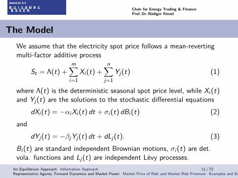
The ModelWe assume that the electricity spot price follows a mean-revertingmulti-factor additive process
St = Λ(t) +m∑
i=1Xi (t) +
n∑j=1
Yj(t) (1)
where Λ(t) is the deterministic seasonal spot price level, while Xi (t)and Yj(t) are the solutions to the stochastic differential equations
dXi (t) = −αiXi (t) dt + σi (t) dBi (t) (2)and
dYj(t) = −βjYj(t) dt + dLj(t). (3)Bi (t) are standard independent Brownian motions, σi (t) are det.vola. functions and Lj(t) are independent Lévy processes.
An Equilibrium Approach Information Approach 11 / 72Representative Agents, Forward Dynamics and Market Power Market Price of Risk and Market Risk Premium Examples and Empirical Evidence

Chair for Energy Trading & FinanceProf. Dr. Rüdiger Kiesel
The Model
The processes Yj(t) are zero-mean reverting processes responsiblefor the spikes or large deviations which revert at a fast rate βj > 0.
Xi (t) are zero-mean reverting processes that account for the normalvariations in the spot price evolution with lower degree ofmean-reversion αi > 0.
An Equilibrium Approach Information Approach 12 / 72Representative Agents, Forward Dynamics and Market Power Market Price of Risk and Market Risk Premium Examples and Empirical Evidence
Chair for Energy Trading & FinanceProf. Dr. Rüdiger Kiesel
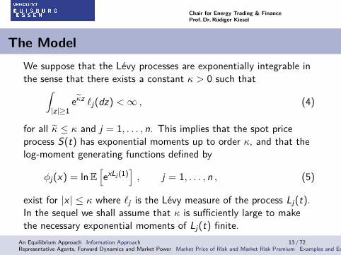
The ModelWe suppose that the Lévy processes are exponentially integrable inthe sense that there exists a constant κ > 0 such that∫
|z|≥1eκz `j(dz) <∞ , (4)
for all κ ≤ κ and j = 1, . . . , n. This implies that the spot priceprocess S(t) has exponential moments up to order κ, and that thelog-moment generating functions defined by
φj(x) = lnE[exLj (1)
], j = 1, . . . , n , (5)
exist for |x | ≤ κ where `j is the Lévy measure of the process Lj(t).In the sequel we shall assume that κ is sufficiently large to makethe necessary exponential moments of Lj(t) finite.
An Equilibrium Approach Information Approach 13 / 72Representative Agents, Forward Dynamics and Market Power Market Price of Risk and Market Risk Premium Examples and Empirical Evidence
Chair for Energy Trading & FinanceProf. Dr. Rüdiger Kiesel
Indifference Prices
Assume that the producer will deliver the spot over the timeinterval [T1,T2].
He has the choice to deliver the production in the spot market,where he faces uncertainty in the prices over the delivery period, orto sell a forward contract with delivery over the same period.
The producer takes this decision at time t ≤ T1.
An Equilibrium Approach Information Approach 14 / 72Representative Agents, Forward Dynamics and Market Power Market Price of Risk and Market Risk Premium Examples and Empirical Evidence
Chair for Energy Trading & FinanceProf. Dr. Rüdiger Kiesel
Indifference Prices
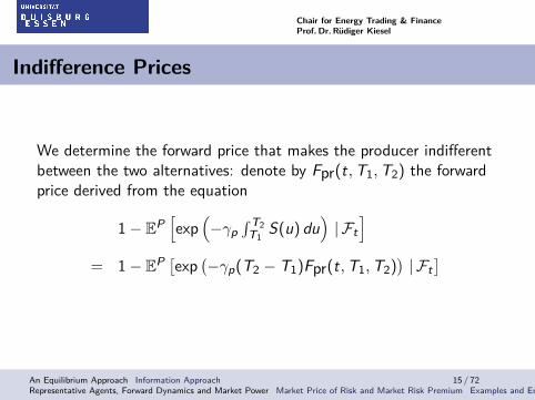
We determine the forward price that makes the producer indifferentbetween the two alternatives: denote by Fpr(t,T1,T2) the forwardprice derived from the equation
1− EP[exp
(−γp
∫ T2T1
S(u) du)| Ft
]= 1− EP [exp (−γp(T2 − T1)Fpr(t,T1,T2)
)| Ft
]
An Equilibrium Approach Information Approach 15 / 72Representative Agents, Forward Dynamics and Market Power Market Price of Risk and Market Risk Premium Examples and Empirical Evidence
Chair for Energy Trading & FinanceProf. Dr. Rüdiger Kiesel
Indifference Prices
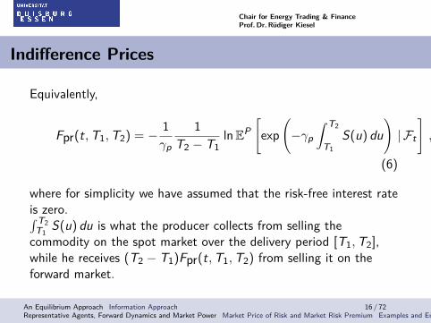
Equivalently,
Fpr(t,T1,T2) = − 1γp
1T2 − T1
lnEP[exp
(−γp
∫ T2
T1S(u) du
)| Ft
],
(6)
where for simplicity we have assumed that the risk-free interest rateis zero.∫ T2
T1S(u) du is what the producer collects from selling the
commodity on the spot market over the delivery period [T1,T2],while he receives (T2 − T1)Fpr(t,T1,T2) from selling it on theforward market.
An Equilibrium Approach Information Approach 16 / 72Representative Agents, Forward Dynamics and Market Power Market Price of Risk and Market Risk Premium Examples and Empirical Evidence
Chair for Energy Trading & FinanceProf. Dr. Rüdiger Kiesel
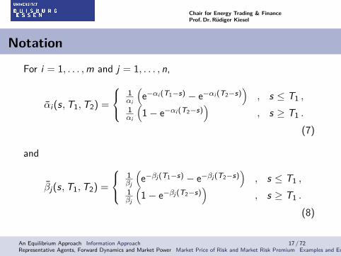
Notation
For i = 1, . . . ,m and j = 1, . . . , n,
αi (s,T1,T2) =
1αi
(e−αi (T1−s) − e−αi (T2−s)
), s ≤ T1 ,
1αi
(1− e−αi (T2−s)
), s ≥ T1 .
(7)
and
βj(s,T1,T2) =
1βj
(e−βj (T1−s) − e−βj (T2−s)
), s ≤ T1 ,
1βj
(1− e−βj (T2−s)
), s ≥ T1 .
(8)
An Equilibrium Approach Information Approach 17 / 72Representative Agents, Forward Dynamics and Market Power Market Price of Risk and Market Risk Premium Examples and Empirical Evidence
Chair for Energy Trading & FinanceProf. Dr. Rüdiger Kiesel
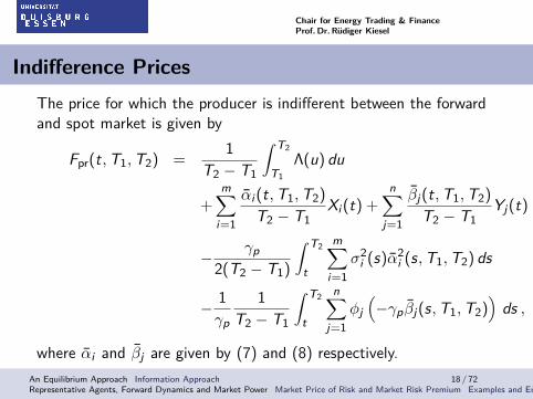
Indifference PricesThe price for which the producer is indifferent between the forwardand spot market is given by
Fpr(t,T1,T2) =1
T2 − T1
∫ T2
T1Λ(u) du
+m∑
i=1
αi (t,T1,T2)
T2 − T1Xi (t) +
n∑j=1
βj(t,T1,T2)
T2 − T1Yj(t)
− γp2(T2 − T1)
∫ T2
t
m∑i=1
σ2i (s)α2
i (s,T1,T2) ds
− 1γp
1T2 − T1
∫ T2
t
n∑j=1
φj(−γpβj(s,T1,T2)
)ds ,
where αi and βj are given by (7) and (8) respectively.An Equilibrium Approach Information Approach 18 / 72Representative Agents, Forward Dynamics and Market Power Market Price of Risk and Market Risk Premium Examples and Empirical Evidence

Chair for Energy Trading & FinanceProf. Dr. Rüdiger Kiesel
Proof – Indifference Price
We calculate the conditional expectation in (6). First observe that∫ T2
T1S(u) du =
∫ T2
T1Λ(u) du +
∫ T2
T1X (u) du +
∫ T2
T1Y (u) du .
An Equilibrium Approach Information Approach 19 / 72Representative Agents, Forward Dynamics and Market Power Market Price of Risk and Market Risk Premium Examples and Empirical Evidence
Chair for Energy Trading & FinanceProf. Dr. Rüdiger Kiesel
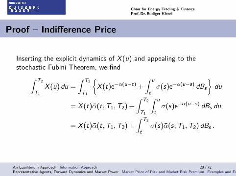
Proof – Indifference Price
Inserting the explicit dynamics of X (u) and appealing to thestochastic Fubini Theorem, we find∫ T2
T1X (u) du =
∫ T2
T1
{X (t)e−α(u−t) +
∫ u
tσ(s)e−α(u−s) dBs
}du
= X (t)α(t,T1,T2) +
∫ T2
T1
∫ u
tσ(s)e−α(u−s) dBs du
= X (t)α(t,T1,T2) +
∫ T2
tσ(s)α(s,T1,T2) dBs .
An Equilibrium Approach Information Approach 20 / 72Representative Agents, Forward Dynamics and Market Power Market Price of Risk and Market Risk Premium Examples and Empirical Evidence

Chair for Energy Trading & FinanceProf. Dr. Rüdiger Kiesel
Proof – Indifference Price
A similar calculation for∫ T2
T1Y (u) du yields,
∫ T2
T1Y (u)du = Y (t)β(t,T1,T2) +
∫ T2
tβ(s,T1,T2) dL(s) .
An Equilibrium Approach Information Approach 21 / 72Representative Agents, Forward Dynamics and Market Power Market Price of Risk and Market Risk Premium Examples and Empirical Evidence
Chair for Energy Trading & FinanceProf. Dr. Rüdiger Kiesel
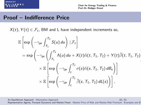
Proof – Indifference Price
X (t),Y (t) ∈ Ft , BM and L have independent increments so,
E[exp
(−γpr
∫ T2
T1S(u) du
)| Ft
]
= exp(−γpr
(∫ T2
T1Λ(u) du + X (t)α(t,T1,T2) + Y (t)β(t,T1,T2)
))
× E[exp
(−γpr
∫ T2
tσ(s)α(s,T1,T2) dBs
)]
× E[exp
(−γpr
∫ T2
tβ(s,T1,T2) dL(s)
)],
An Equilibrium Approach Information Approach 22 / 72Representative Agents, Forward Dynamics and Market Power Market Price of Risk and Market Risk Premium Examples and Empirical Evidence
Chair for Energy Trading & FinanceProf. Dr. Rüdiger Kiesel
Proof – Indifference Price
E[exp
(−γpr
∫ T2
T1S(u) du
)| Ft
]
= exp(−γpr
(∫ T2
T1Λ(u) du + X (t)α(t,T1,T2) + Y (t)β(t,T1,T2)
))
× exp(12γ
2pr
∫ T2
tσ2(s)α2(s,T1,T2) ds
)
× exp(∫ T2
tφ(−γprβ(s,T1,T2)) ds
).
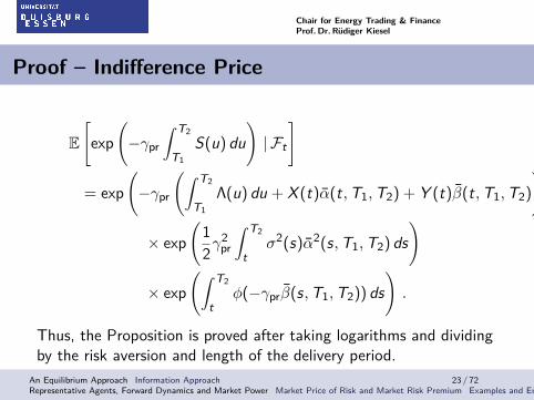
Thus, the Proposition is proved after taking logarithms and dividingby the risk aversion and length of the delivery period.
An Equilibrium Approach Information Approach 23 / 72Representative Agents, Forward Dynamics and Market Power Market Price of Risk and Market Risk Premium Examples and Empirical Evidence
Chair for Energy Trading & FinanceProf. Dr. Rüdiger Kiesel
Indifference Price – Jumps
Suppose Lj(t) is a process of only positive jumps.
Then, the log-moment generating function φj(x) of Lj(t) is anincreasing function with φj(0) = 0.
Thus, when x < 0, φj(x) < 0, and since βj is positive, we have thatthe argument of φj(·) in the indifference price of the producer isnegative, and thus the jump process Lj(t) causes an increase in theindifference forward price.
Intuitively, positive price spikes work to the advantage of theproducer, and he will be reluctant to enter forward contracts thatmiss such opportunities.
An Equilibrium Approach Information Approach 24 / 72Representative Agents, Forward Dynamics and Market Power Market Price of Risk and Market Risk Premium Examples and Empirical Evidence
Chair for Energy Trading & FinanceProf. Dr. Rüdiger Kiesel
Indifference Price – Jumps
On the other hand, if Lj(t) only exhibit negative jumps, we see thatthe indifference price is pushed downwards.
Intuitively, the producer is willing to accept lower forward pricessince there is a risk of price drops in the spot market.
An Equilibrium Approach Information Approach 25 / 72Representative Agents, Forward Dynamics and Market Power Market Price of Risk and Market Risk Premium Examples and Empirical Evidence
Chair for Energy Trading & FinanceProf. Dr. Rüdiger Kiesel
Indifference Price – Retailer
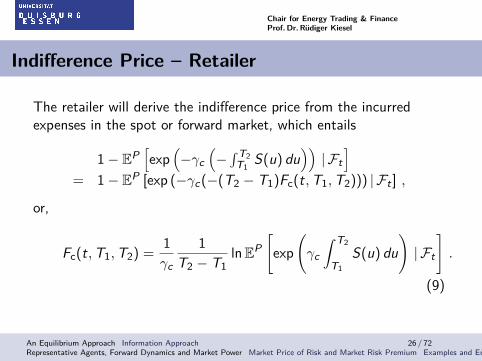
The retailer will derive the indifference price from the incurredexpenses in the spot or forward market, which entails
1− EP[exp
(−γc
(−∫ T2
T1S(u) du
))| Ft
]= 1− EP [exp (−γc(−(T2 − T1)Fc(t,T1,T2))) | Ft ] ,
or,
Fc(t,T1,T2) =1γc
1T2 − T1
lnEP[exp
(γc
∫ T2
T1S(u) du
)| Ft
].
(9)
An Equilibrium Approach Information Approach 26 / 72Representative Agents, Forward Dynamics and Market Power Market Price of Risk and Market Risk Premium Examples and Empirical Evidence
Chair for Energy Trading & FinanceProf. Dr. Rüdiger Kiesel
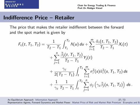
Indifference Price – RetailerThe price that makes the retailer indifferent between the forwardand the spot market is given by
Fc(t,T1,T2) =1
T2 − T1
∫ T2
T1Λ(u) du +
m∑i=1
αi (t,T1,T2)
T2 − T1Xi (t)
+n∑
j=1
βj(t,T1,T2)
T2 − T1Yj(t)
+γc
2(T2 − T1)
∫ T2
t
m∑i=1
σ2i (s)α2
i (s,T1,T2) ds
+1γc
1T2 − T1
∫ T2
t
n∑j=1
φj(γc βj(s,T1,T2)
)ds .
An Equilibrium Approach Information Approach 27 / 72Representative Agents, Forward Dynamics and Market Power Market Price of Risk and Market Risk Premium Examples and Empirical Evidence
Chair for Energy Trading & FinanceProf. Dr. Rüdiger Kiesel
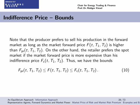
Indifference Price – Bounds
Note that the producer prefers to sell his production in the forwardmarket as long as the market forward price F (t,T1,T2) is higherthan Fpr(t,T1,T2). On the other hand, the retailer prefers the spotmarket if the market forward price is more expensive than hisindifference price Fc(t,T1,T2). Thus, we have the bounds
Fpr(t,T1,T2) ≤ F (t,T1,T2) ≤ Fc(t,T1,T2) . (10)
An Equilibrium Approach Information Approach 28 / 72Representative Agents, Forward Dynamics and Market Power Market Price of Risk and Market Risk Premium Examples and Empirical Evidence
Chair for Energy Trading & FinanceProf. Dr. Rüdiger Kiesel
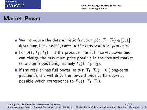
Market Power
We introduce the deterministic function p(t,T1,T2) ∈ [0, 1]describing the market power of the representative producer.For p(t,T1,T2) = 1 the producer has full market power andcan charge the maximum price possible in the forward market(short-term positions), namely Fc(t,T1,T2).If the retailer has full power, ie p(t,T1,T2) = 0 (long-termpositions), she will drive the forward price as far down aspossible which corresponds to Fpr(t,T1,T2).
An Equilibrium Approach Information Approach 29 / 72Representative Agents, Forward Dynamics and Market Power Market Price of Risk and Market Risk Premium Examples and Empirical Evidence
Chair for Energy Trading & FinanceProf. Dr. Rüdiger Kiesel
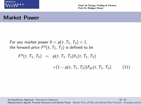
Market Power
For any market power 0 < p(t,T1,T2) < 1,the forward price F p(t,T1,T2) is defined to be
F p(t,T1,T2) = p(t,T1,T2)Fc(t,T1,T2)
+(1− p(t,T1,T2))Fpr(t,T1,T2). (11)
An Equilibrium Approach Information Approach 30 / 72Representative Agents, Forward Dynamics and Market Power Market Price of Risk and Market Risk Premium Examples and Empirical Evidence
Chair for Energy Trading & FinanceProf. Dr. Rüdiger Kiesel
Market Power
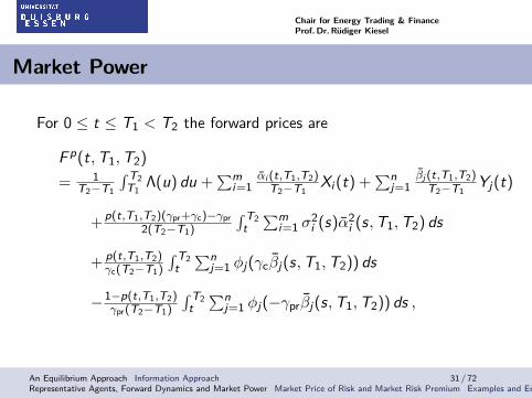
For 0 ≤ t ≤ T1 < T2 the forward prices are
F p(t,T1,T2)
= 1T2−T1
∫ T2T1
Λ(u) du +∑m
i=1αi (t,T1,T2)
T2−T1Xi (t) +
∑nj=1
βj (t,T1,T2)T2−T1
Yj(t)
+p(t,T1,T2)(γpr+γc)−γpr2(T2−T1)
∫ T2t∑m
i=1 σ2i (s)α2
i (s,T1,T2) ds
+ p(t,T1,T2)γc(T2−T1)
∫ T2t∑n
j=1 φj(γcβj(s,T1,T2)) ds
−1−p(t,T1,T2)γpr(T2−T1)
∫ T2t∑n
j=1 φj(−γprβj(s,T1,T2)) ds ,
An Equilibrium Approach Information Approach 31 / 72Representative Agents, Forward Dynamics and Market Power Market Price of Risk and Market Risk Premium Examples and Empirical Evidence
Chair for Energy Trading & FinanceProf. Dr. Rüdiger Kiesel
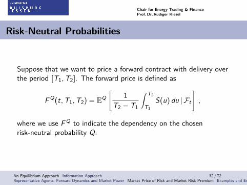
Risk-Neutral Probabilities
Suppose that we want to price a forward contract with delivery overthe period [T1,T2]. The forward price is defined as
F Q(t,T1,T2) = EQ[
1T2 − T1
∫ T2
T1S(u) du | Ft
],
where we use F Q to indicate the dependency on the chosenrisk-neutral probability Q.
An Equilibrium Approach Information Approach 32 / 72Representative Agents, Forward Dynamics and Market Power Market Price of Risk and Market Risk Premium Examples and Empirical Evidence
Chair for Energy Trading & FinanceProf. Dr. Rüdiger Kiesel
Risk-Neutral Probabilities
We parameterize the market price of risk by introducing aprobability measure Qθ := QB × QL, where QB is a Girsanovtransform of the Brownian motions Bi (t), QL is an Esschertransform of the jump processes Lj(t), and θ is an Rn+m-valuedfunction describing the market price of risk.
An Equilibrium Approach Information Approach 33 / 72Representative Agents, Forward Dynamics and Market Power Market Price of Risk and Market Risk Premium Examples and Empirical Evidence

Chair for Energy Trading & FinanceProf. Dr. Rüdiger Kiesel
Risk-Neutral Probabilities -Brownian Motions
For t ≤ T , with T ≥ T2 being a finite time horizon encapsulatingall the delivery periods in the market, let the probability QB havethe density process
ZB(t) = exp(−∫ t
0
m∑i=1
θB,i (t)
σi (s)dBi (s)− 1
2
∫ t
0
m∑i=1
θ2B,i (s)
σ2i (s)
ds),
where we have supposed that the functions θB,i/σi , i = 1, . . . ,m,are square integrable over [0,T ].
An Equilibrium Approach Information Approach 34 / 72Representative Agents, Forward Dynamics and Market Power Market Price of Risk and Market Risk Premium Examples and Empirical Evidence
Chair for Energy Trading & FinanceProf. Dr. Rüdiger Kiesel
Risk-Neutral Probabilities -Brownian Motions
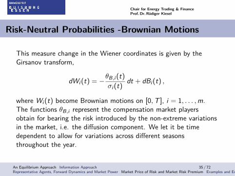
This measure change in the Wiener coordinates is given by theGirsanov transform,
dWi (t) = −θB,i (t)
σi (t)dt + dBi (t) ,
where Wi (t) become Brownian motions on [0,T ], i = 1, . . . ,m.The functions θB,i represent the compensation market playersobtain for bearing the risk introduced by the non-extreme variationsin the market, i.e. the diffusion component. We let it be timedependent to allow for variations across different seasonsthroughout the year.
An Equilibrium Approach Information Approach 35 / 72Representative Agents, Forward Dynamics and Market Power Market Price of Risk and Market Risk Premium Examples and Empirical Evidence
Chair for Energy Trading & FinanceProf. Dr. Rüdiger Kiesel
Risk-Neutral Probabilities -Brownian Motions
This Girsanov change gives the dynamics (for 1 ≤ i ≤ m)
dXi (t) = (θB,i (t)− αiXi (t)) dt + σi (t) dWi (t) ,
and thus we have added a time-dependent level of mean-reversionto the processes Xi (t).
An Equilibrium Approach Information Approach 36 / 72Representative Agents, Forward Dynamics and Market Power Market Price of Risk and Market Risk Premium Examples and Empirical Evidence
Chair for Energy Trading & FinanceProf. Dr. Rüdiger Kiesel
Risk-Neutral Probabilities -Lévy Processe
Further, define for bounded functions θL,j , j = 1, . . . , n,
ZL(t) = exp
∫ t
0
n∑j=1
θL,j(s) dLj(s)−∫ t
0
n∑j=1
φj(θL,j(s)) ds
,
for t ≤ T2, and let the density process for the Radon-Nikodymderivative of the measure change in the jump component be
dQLdP
∣∣∣∣Ft
= ZL(t) .
This is the so-called Esscher transform, and the time dependentfunctions θL,j(t) are the market prices of jump risk.
An Equilibrium Approach Information Approach 37 / 72Representative Agents, Forward Dynamics and Market Power Market Price of Risk and Market Risk Premium Examples and Empirical Evidence
Chair for Energy Trading & FinanceProf. Dr. Rüdiger Kiesel
Risk-Neutral Probabilities
We let θ := (θB, θL), where θB := (θB,i )mi=1 and θL := (θL,j)
nj=1.
The density process of the probability Qθ becomesZ (t) := ZB(t)ZL(t).
We denote by EQθ the expectation with respect to the probabilitymeasure Qθ.
An Equilibrium Approach Information Approach 38 / 72Representative Agents, Forward Dynamics and Market Power Market Price of Risk and Market Risk Premium Examples and Empirical Evidence
Chair for Energy Trading & FinanceProf. Dr. Rüdiger Kiesel
Forward Price
The forward price F θ(t,T1,T2) is given by
F θ(t,T1,T2)
= 1T2−T1
∫ T2T1
Λ(u) du +∑m
i=1αi (t,T1,T2)
T2−T1Xi (t) +
∑nj=1
βj (t,T1,T2)T2−T1
Yj(t)
+∫ T2
t∑m
i=1 θB,i (s) αi (s,T1,T2)T2−T1
ds
+∫ T2
t∑n
j=1 φ′j(θL,j(s))
βj (s,T1,T2)T2−T1
ds .
for 0 ≤ t ≤ T1 < T2.
An Equilibrium Approach Information Approach 39 / 72Representative Agents, Forward Dynamics and Market Power Market Price of Risk and Market Risk Premium Examples and Empirical Evidence

Chair for Energy Trading & FinanceProf. Dr. Rüdiger Kiesel
Forward Price – Proof
The explicit representation of X (t) under Qθ is
X (u) = X (t)eα(u−t)+
∫ u
tθB(s)e−α(u−s) ds+
∫ u
tσ(u)e−α(u−s) dW (s) ,
for u ≥ t.
An Equilibrium Approach Information Approach 40 / 72Representative Agents, Forward Dynamics and Market Power Market Price of Risk and Market Risk Premium Examples and Empirical Evidence
Chair for Energy Trading & FinanceProf. Dr. Rüdiger Kiesel
Forward Price – Proof
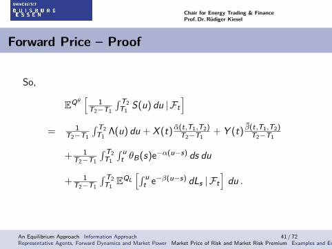
So,
EQθ[
1T2−T1
∫ T2T1
S(u) du | Ft]
= 1T2−T1
∫ T2T1
Λ(u) du + X (t) α(t,T1,T2)T2−T1
+ Y (t) β(t,T1,T2)T2−T1
+ 1T2−T1
∫ T2T1
∫ ut θB(s)e−α(u−s) ds du
+ 1T2−T1
∫ T2T1
EQL[∫ u
t e−β(u−s) dLs | Ft]
du .
An Equilibrium Approach Information Approach 41 / 72Representative Agents, Forward Dynamics and Market Power Market Price of Risk and Market Risk Premium Examples and Empirical Evidence
Chair for Energy Trading & FinanceProf. Dr. Rüdiger Kiesel
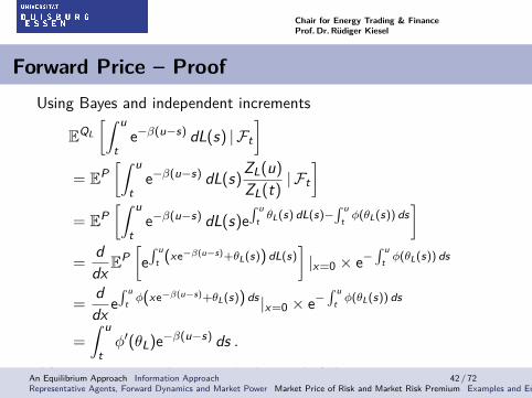
Forward Price – ProofUsing Bayes and independent increments
EQL
[∫ u
te−β(u−s) dL(s) | Ft
]= EP
[∫ u
te−β(u−s) dL(s)
ZL(u)
ZL(t)| Ft
]= EP
[∫ u
te−β(u−s) dL(s)e
∫ ut θL(s) dL(s)−
∫ ut φ(θL(s)) ds
]=
ddx E
P[e∫ u
t (xe−β(u−s)+θL(s)) dL(s)]|x=0 × e−
∫ ut φ(θL(s)) ds
=ddx e
∫ ut φ(xe−β(u−s)+θL(s)) ds |x=0 × e−
∫ ut φ(θL(s)) ds
=
∫ u
tφ′(θL)e−β(u−s) ds .
After reorganizing the integrals the result follows.An Equilibrium Approach Information Approach 42 / 72Representative Agents, Forward Dynamics and Market Power Market Price of Risk and Market Risk Premium Examples and Empirical Evidence
Chair for Energy Trading & FinanceProf. Dr. Rüdiger Kiesel
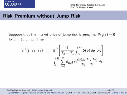
Risk Premium without Jump Risk
Suppose that the market price of jump risk is zero, i.e. θL,j(s) = 0for j = 1, . . . , n. Then
F θ(t,T1,T2) = EP[
1T2 − T1
∫ T2
T1S(u) du | Ft
]
+
∫ T2
t
m∑i=1
θB,i (s)αi (s,T1,T2)
T2 − T1ds .
An Equilibrium Approach Information Approach 43 / 72Representative Agents, Forward Dynamics and Market Power Market Price of Risk and Market Risk Premium Examples and Empirical Evidence

Chair for Energy Trading & FinanceProf. Dr. Rüdiger Kiesel
Risk Premium without Jump Risk
Thus, we see that when market players are not compensated forbearing jump risk, the market risk premium is positive as long as
π(t,T1,T2) =
∫ T2
t
m∑i=1
θB,i (s)αi (s,T1,T2)
T2 − T1ds
is positive.
An Equilibrium Approach Information Approach 44 / 72Representative Agents, Forward Dynamics and Market Power Market Price of Risk and Market Risk Premium Examples and Empirical Evidence
Chair for Energy Trading & FinanceProf. Dr. Rüdiger Kiesel
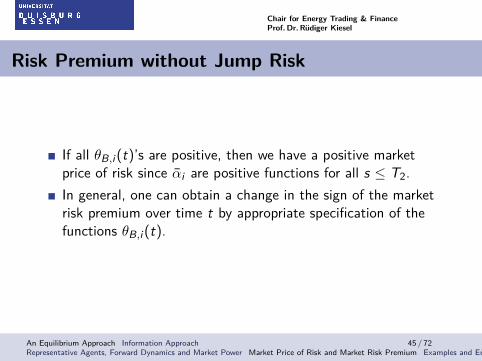
Risk Premium without Jump Risk
If all θB,i (t)’s are positive, then we have a positive marketprice of risk since αi are positive functions for all s ≤ T2.In general, one can obtain a change in the sign of the marketrisk premium over time t by appropriate specification of thefunctions θB,i (t).
An Equilibrium Approach Information Approach 45 / 72Representative Agents, Forward Dynamics and Market Power Market Price of Risk and Market Risk Premium Examples and Empirical Evidence
Chair for Energy Trading & FinanceProf. Dr. Rüdiger Kiesel
Example: Model Specification
We consider a forward market consisting of 52 contracts withweekly delivery. The market power is supposed to be constantp(t,T1,T2) = p ∈ [0, 1]. Assume that the spot model has m = 52diffusion components Xi (t), and one (n = 1) jump componentY (t). Suppose that the seasonal function is
Λ(t) = 150 + 20 cos(2πt/365) ,
and the mean-reversion parameters for the diffusion components areαi = 0.067/i , with volatility σi = 0.3/
√i , for i = 1, . . . , 52.
An Equilibrium Approach Information Approach 46 / 72Representative Agents, Forward Dynamics and Market Power Market Price of Risk and Market Risk Premium Examples and Empirical Evidence
Chair for Energy Trading & FinanceProf. Dr. Rüdiger Kiesel
Model Specification
We mimic here a sequence of mean-reverting processes withdecreasing speeds of mean reversion and with decreasingvolatility.The speed of mean reversion equal to 0.067 means that ashock will be halved over 10 days.The jump process is driven by L(t) = ηN(t), where N(t) is aPoisson process with intensity λ and the jump size is constant,equal to η.
An Equilibrium Approach Information Approach 47 / 72Representative Agents, Forward Dynamics and Market Power Market Price of Risk and Market Risk Premium Examples and Empirical Evidence
Chair for Energy Trading & FinanceProf. Dr. Rüdiger Kiesel
Model Specification
The mean-reversion for the jump component is β = 0.5,meaning that a jump will, on average, revert back in two days.We have a combination of slow mean reverting normalvariations and fast mean reverting spikes in the spot market.The frequency of spikes is set to λ = 2/365, i.e. two spikes, onaverage, per year.
An Equilibrium Approach Information Approach 48 / 72Representative Agents, Forward Dynamics and Market Power Market Price of Risk and Market Risk Premium Examples and Empirical Evidence
Chair for Energy Trading & FinanceProf. Dr. Rüdiger Kiesel
Model Specification
Time t = 0 corresponds to January 1, and we assume that theinitial spot price is S(0) = 172.We let X1(0) = 2, and Xi (0) = Y (0) = 0 for i = 2, . . . , 52 toachieve this.The risk aversion coefficients of the producer and retailer areset equal to γc = γpr = 0.5.We derive forward curves for weakly settled forward contractsover a year.
An Equilibrium Approach Information Approach 49 / 72Representative Agents, Forward Dynamics and Market Power Market Price of Risk and Market Risk Premium Examples and Empirical Evidence
Chair for Energy Trading & FinanceProf. Dr. Rüdiger Kiesel
Indifference price with forward curves for positivejumpsvanish as a consequence of mean reversion and the consumer will have more power driving
the market risk premium below zero. To illustrate this particular example with p = 0.5 we
0 10 20 30 40 50
50
100
150
200
250
300Pos itive jumps
week of delivery
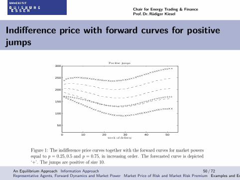
Figure 1: The indifference price curves together with the forward curves for market powersequal to p = 0.25, 0.5 and p = 0.75, in increasing order. The forecasted curve is depicted‘+’. The jumps are positive of size 10.
have plotted the difference of the forward curve with market power 0.25 and the forecastedcurve in Fig. 2. For the contracts with delivery up to approximately week 20, the marketpremium is positive. The premium decreases with time to delivery, and becomes negativein the medium and long end. in the long end.
Turning our attention to the case of negative jumps, we observe the reverse picture.Suppose that jumps sizes are fixed at η = −10. Fig. 3 shows the corresponding forward andindifference curves together with the forecasted price. We observe first of all that all curvesare shifted downwards, indicating that the producer is willing to accept lower forward pricesto hedge the possibility of sudden drops in prices. In the short-term we observe, for allcases of market power, that the forecasted spot price is above forward prices, i.e. negativemarket risk premium. In the long-term, only when producer’s market power is high, that is0.75, we have the situation where the forecasted curve is below the forward curve signalingthat the consumer bears a positive risk premium. Moreover, Fig. 4 shows the differencebetween the forward curve and the forecasted curve when the producer’s market power isp = 0.75.
We now proceed to analyze more closely the implications of jumps and normal vari-ations of the model. We consider the case with m = n = 1 and constant market powerp(t, T1, T2) = p for p ∈ [0, 1]. Further, let L(t) = N(t), a Poisson process with constantjump intensity λ > 0. Note that this model has only two factors, and in general it willnot give an arbitrage-free forward curve dynamics for a market which trades in contractswith many different delivery periods. However, this simplification provides us with some
16
An Equilibrium Approach Information Approach 50 / 72Representative Agents, Forward Dynamics and Market Power Market Price of Risk and Market Risk Premium Examples and Empirical Evidence
Chair for Energy Trading & FinanceProf. Dr. Rüdiger Kiesel
Market risk premium – positive jumps
Market clearing forward prices are increasing with increasingmarket power, since the producer will command higher priceswith more power.For a low market power of 0.25, we observe that the forecastedprice curve is below the forward curve in the shorter end, whilein the medium to long end we see the opposite.This corresponds to a positive market risk premium in theshorter end, whereas it becomes negative in the medium andlonger end.The retailer wishes to avoid upward jumps in the price and is,even for a weak producer, willing to accept a positive marketrisk premium in the short end. In the long end, the effect ofjumps vanish as a consequence of mean reversion, so theretailer will have more power.
An Equilibrium Approach Information Approach 51 / 72Representative Agents, Forward Dynamics and Market Power Market Price of Risk and Market Risk Premium Examples and Empirical Evidence
Chair for Energy Trading & FinanceProf. Dr. Rüdiger Kiesel
Market risk premium – positive jumps
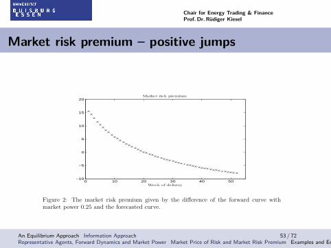
To illustrate this particular example we have plotted the differenceof the forward curve with market power 0.25 and the forecastedcurve. For the contracts with delivery up to approximately week 20,the market premium is positive. The premium decreases with timeto delivery, and becomes negative in the medium and long end.
An Equilibrium Approach Information Approach 52 / 72Representative Agents, Forward Dynamics and Market Power Market Price of Risk and Market Risk Premium Examples and Empirical Evidence
Chair for Energy Trading & FinanceProf. Dr. Rüdiger Kiesel
Market risk premium – positive jumps
0 10 20 30 40 50−10
−5
0
5
10
15
20Market risk premium
Week of delivery
Figure 2: The market risk premium given by the difference of the forward curve withmarket power 0.25 and the forecasted curve.
insight into how the sign of the market risk premium may change, and we include it withthe assumption that we have one forward contract with delivery period [T1, T2] traded inthe market.
Consider equation (4.3). One way to solve this is to separate the Wiener and jumppart, and solve the two resulting equations. We find the solution
θB(t, T1, T2) =1
2(p(γpr + γc)− γpr) σ
2(t)α(t, T1, T2) , (4.4)
for t ≤ T2. Note that the sign of θB depends on the sign of p(γpr + γc) − γpr, since σ2(t)and α(t, T1, T2) are positive. We have a negative market price of risk θB whenever
p <γpr
γpr + γc. (4.5)
If for instance γpr = γc, the market price of risk θB becomes negative whenever p < 0.5,which corresponds to the consumer being the strongest. If the producer is strongest, iep > 0.5, he is the superior power in forming prices and the market price of risk becomespositive. If γpr 6= γc, the market power needs to be less than the relative risk aversion ofthe producer against the total risk aversion for θB to be negative.
Let us consider the market price of jump risk. Since L(t) is assumed to be a Poissonprocess, the log-moment generating function is given by
φ(x) = λ(ex − 1) and φ′(x) = λex .
Note thatφ′(θL(t))− φ′(0) = λ(eθL(t) − 1)
17
An Equilibrium Approach Information Approach 53 / 72Representative Agents, Forward Dynamics and Market Power Market Price of Risk and Market Risk Premium Examples and Empirical Evidence
Chair for Energy Trading & FinanceProf. Dr. Rüdiger Kiesel
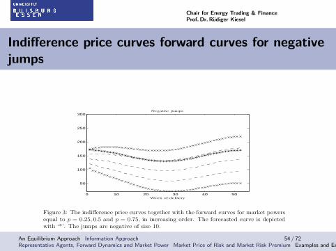
Indifference price curves forward curves for negativejumps
0 10 20 30 40 50
50
100
150
200
250
300Negative jumps
Week of delivery
Figure 3: The indifference price curves together with the forward curves for market powersequal to p = 0.25, 0.5 and p = 0.75, in increasing order. The forecasted curve is depictedwith ‘*’. The jumps are negative of size 10.
which is positive whenever θL(t) > 0, and negative if θL(t) < 0, as expected following theinterpretation of Corollary 4.3. The equation for the jump risk derived from splitting (4.3)into two equations becomes (after differentiating with respect to t)
λeθL(t)β(t, T1, T2) =p
γcλ(eγcβ(t,T1,T2) − 1)− 1− p
γprλ(e−γprβ(t,T1,T2) − 1) .
Or, equivalently,
β(t, T1, T2)eθL(t,T1,T2) =
p
γc(eγcβ(t,T1,T2) − 1) +
1− p
γpr(1− e−γprβ(t,T1,T2)) . (4.6)
Note that the right-hand-side of (4.6) is positive since β(t, T1, T2) > 0. Thus, the marketprice of jump risk is negative whenever
p
γc(eγcβ(t,T1,T2) − 1) +
1− p
γpr(1− e−γprβ(t,T1,T2)) < β(t, T1, T2) ,
and positive otherwise. The following Lemma is helpful in understanding when the marketprice of jump risk is negative.
Lemma 4.4. The non-negative function f : R+ 7→ R+ defined by
f(z) =p
γc(eγcz − 1) +
1− p
γpr(1− e−γprz) ,
satisfies f(z) ≥ z for all z ≥ 0 when
p >γpr
γpr + γc.
18
An Equilibrium Approach Information Approach 54 / 72Representative Agents, Forward Dynamics and Market Power Market Price of Risk and Market Risk Premium Examples and Empirical Evidence
Chair for Energy Trading & FinanceProf. Dr. Rüdiger Kiesel
Market risk premium – negative jumps
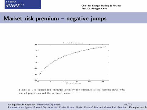
We observe that all curves are shifted downwards, indicatingthat the producer is willing to accept lower forward prices tohedge the possibility of sudden drops in prices.In the short-term we observe, for all cases of market power,that the forecasted spot price is above forward prices, i.e.negative market risk premium.In the long-term, only when producer’s market power is high,that is 0.75, we have the situation where the forecasted curveis below the forward curve signaling that the retailer bears apositive risk premium.
An Equilibrium Approach Information Approach 55 / 72Representative Agents, Forward Dynamics and Market Power Market Price of Risk and Market Risk Premium Examples and Empirical Evidence
Chair for Energy Trading & FinanceProf. Dr. Rüdiger Kiesel
Market risk premium – negative jumps
0 10 20 30 40 50−20
−15
−10
−5
0
5
10Market risk premium
Week of delivery
Figure 4: The market risk premium given by the difference of the forward curve withmarket power 0.75 and the forecasted curve.
Moreover, if
p <γpr
γpr + γc,
then f(z) < z for z ≤ z0, and f(z) ≥ z otherwise, where z0 is defined by f(z) = z.
Proof. Observe that f(0) = 0, and f(z) → ∞ whenever z → ∞. Moreover, f is monoton-ically increasing since
f ′(z) = peγcz + (1− p)e−γcz ≥ 0 .
Consider f ′′(z):f ′′(z) = pγce
γcz − (1− p)γpre−γprz ,
which is positive whenever p > γpr/(γc+ γpr). In that case, f ′(z) is an increasing function,and since f ′(0) = 1, we find that f ′(z) ≥ 1, and therefore f(z) ≥ z for all z ≥ 0. Thisproves the first claim. When p < γpr/(γc + γpr), we will have that f ′′(z) < 0 for z ≤ z,where z is some positive constant, while f ′′(z) > 0 elsewhere. Thus, f ′(z) is decreasing,and next increasing. Since it goes to infinity as an exponential, we need to have that thereexists z0 > 0 for which f(z0) = z0. The second claim follows.
Let z = β(t, T1, T2) in the Lemma above, and recall that by the definition of β(t, T1, T2)it is increasing in t ≤ T1 and decreasing in T1 < t ≤ T2. Its maximum is in t = T1, where ittakes the value β(T1, T1, T2) = (1−e−β(T2−T1))/β. If this maximum is less than z0, the jumprisk θL(t, T1, T2) will be negative for all t ≤ T2. Consider the situation where the maximumis greater than z0. Observe that β(0, T1, T2) = (e−βT1 − e−βT2)/β and β(T2, T1, T2) = 0. Ifβ(0, T1, T2) ≥ z0, there exists one t0 such that β(t0, T1, T2) = z0. In this case we find thatθL(t, T1, T2) > 0 for t < t0, and θL(t, T1, T2) < 0 for t > t0. If β(0, T1, T2) < z0, we have
19
An Equilibrium Approach Information Approach 56 / 72Representative Agents, Forward Dynamics and Market Power Market Price of Risk and Market Risk Premium Examples and Empirical Evidence
Chair for Energy Trading & FinanceProf. Dr. Rüdiger Kiesel
Estimation problems
We need to estimate the physical parameters of our two-factormodel.From forward market data, denoted by F (t,T1,T2), weestimate the risk-aversion coefficients for both producers andretailers and estimate the producer’s market power.
An Equilibrium Approach Information Approach 57 / 72Representative Agents, Forward Dynamics and Market Power Market Price of Risk and Market Risk Premium Examples and Empirical Evidence
Chair for Energy Trading & FinanceProf. Dr. Rüdiger Kiesel
Data used
Spot prices: Phelix base load traded at the EEX.Forward contract prices with delivery periods: monthly,quarterly and yearly.Period covered: January 2 2002 to January 1 2006 with 1461spot price observations.Forward data: 108 contracts with monthly delivery, 35contracts with quarterly delivery and 12 contracts with yearlydelivery.
An Equilibrium Approach Information Approach 58 / 72Representative Agents, Forward Dynamics and Market Power Market Price of Risk and Market Risk Premium Examples and Empirical Evidence
Chair for Energy Trading & FinanceProf. Dr. Rüdiger Kiesel
Spot model specification
We apply the model to
S(t) = Λ(t) + X (t) + Y (t)
where, Λ(t) is the seasonal component,
dX (t) = −αX (t)dt + σdB(t) (12)
where α ≥ 0, σ ≥ 0 and B(t) is a standard Brownian motion,
An Equilibrium Approach Information Approach 59 / 72Representative Agents, Forward Dynamics and Market Power Market Price of Risk and Market Risk Premium Examples and Empirical Evidence
Chair for Energy Trading & FinanceProf. Dr. Rüdiger Kiesel
Spot model specification
dY (t) = −βY (t)dt + dL(t) (13)with β ≥ 0 and
L(t) =
N(t)∑i
Ji (14)
is a compound Poisson process.N(t) is a homogeneous Poisson process with intensity λ and Ji ’sare i.i.d. with exponential density function
f (j) = pλ1e−λ1j1j>0 + (1− p)λ2e−λ2|j|1j<0,
where λ1 > 0 and λ2 > 0 are responsible for the decay of the tailsfor the distribution.We assume that N(t), J and B(t) are independent.An Equilibrium Approach Information Approach 60 / 72
Representative Agents, Forward Dynamics and Market Power Market Price of Risk and Market Risk Premium Examples and Empirical Evidence
Chair for Energy Trading & FinanceProf. Dr. Rüdiger Kiesel
Spot model specification
For the seasonal component we assume
Λ(t) = a0 + a11{t=Su} + a21{t=Mo,Fri} + a31{t=Tu,We,Th} + a41{t=Sa}
+a5 cos[ 6π365 (t + a6)
]+ a7t,
where the indicator function is acting on the different days of theweek.
An Equilibrium Approach Information Approach 61 / 72Representative Agents, Forward Dynamics and Market Power Market Price of Risk and Market Risk Premium Examples and Empirical Evidence
Chair for Energy Trading & FinanceProf. Dr. Rüdiger Kiesel
Risk aversion coefficients
Recall that Fc(t,T1,T2) (upper bound) and Fpr (t,T1,T2) (lowerbound) depend on the choice of γc and γpr , we estimate γpr and γcby minimizing the distance between Fc(t,T1,T2), Fpr (t,T1,T2)and the market prices of forwards F (t,T1,T2), respectively, in thefollowing way.
An Equilibrium Approach Information Approach 62 / 72Representative Agents, Forward Dynamics and Market Power Market Price of Risk and Market Risk Premium Examples and Empirical Evidence
Chair for Energy Trading & FinanceProf. Dr. Rüdiger Kiesel
Risk aversion coefficients
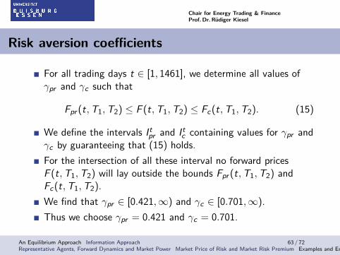
For all trading days t ∈ [1, 1461], we determine all values ofγpr and γc such that
Fpr (t,T1,T2) ≤ F (t,T1,T2) ≤ Fc(t,T1,T2). (15)
We define the intervals Itpr and It
c containing values for γpr andγc by guaranteeing that (15) holds.For the intersection of all these interval no forward pricesF (t,T1,T2) will lay outside the bounds Fpr (t,T1,T2) andFc(t,T1,T2).We find that γpr ∈ [0.421,∞) and γc ∈ [0.701,∞).Thus we choose γpr = 0.421 and γc = 0.701.
An Equilibrium Approach Information Approach 63 / 72Representative Agents, Forward Dynamics and Market Power Market Price of Risk and Market Risk Premium Examples and Empirical Evidence
Chair for Energy Trading & FinanceProf. Dr. Rüdiger Kiesel
Market power and market risk
Recall
p(t,T1,T2) =F (t,T1,T2)− Fpr (t,T1,T2)
Fc(t,T1,T2)− Fpr (t,T1,T2)
and
π(t,T1,T2) = F (t,T1,T2)− EP[
1T2 − T1
∫ T2
T1S(u)du|Ft
].
An Equilibrium Approach Information Approach 64 / 72Representative Agents, Forward Dynamics and Market Power Market Price of Risk and Market Risk Premium Examples and Empirical Evidence
Chair for Energy Trading & FinanceProf. Dr. Rüdiger Kiesel
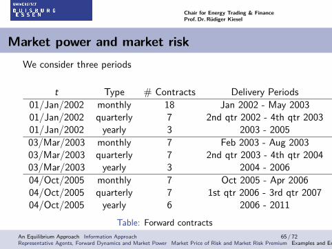
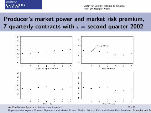
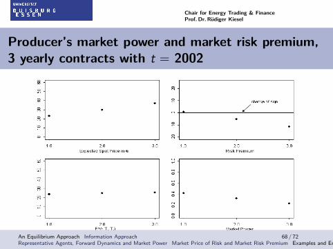
Market power and market riskWe consider three periods
t Type # Contracts Delivery Periods F (t,T1,T2)
01/Jan/2002 monthly 18 Jan 2002 - May 2003 F (2,T1,T2)01/Jan/2002 quarterly 7 2nd qtr 2002 - 4th qtr 2003 F (2,T1,T2)01/Jan/2002 yearly 3 2003 - 2005 F (2,T1,T2)
03/Mar/2003 monthly 7 Feb 2003 - Aug 2003 F (400,T1,T2)03/Mar/2003 quarterly 7 2nd qtr 2003 - 4th qtr 2004 F (400,T1,T2)03/Mar/2003 yearly 3 2004 - 2006 F (400,T1,T2)
04/Oct/2005 monthly 7 Oct 2005 - Apr 2006 F (1373,T1,T2)04/Oct/2005 quarterly 7 1st qtr 2006 - 3rd qtr 2007 F (1373,T1,T2)04/Oct/2005 yearly 6 2006 - 2011 F (1373,T1,T2)
Table: Forward contractsAn Equilibrium Approach Information Approach 65 / 72Representative Agents, Forward Dynamics and Market Power Market Price of Risk and Market Risk Premium Examples and Empirical Evidence

Chair for Energy Trading & FinanceProf. Dr. Rüdiger Kiesel
Producer’s market power and market risk premium,18 monthly contracts with t = January 2 2002
An Equilibrium Approach Information Approach 66 / 72Representative Agents, Forward Dynamics and Market Power Market Price of Risk and Market Risk Premium Examples and Empirical Evidence
Chair for Energy Trading & FinanceProf. Dr. Rüdiger Kiesel
Producer’s market power and market risk premium,7 quarterly contracts with t = second quarter 2002
An Equilibrium Approach Information Approach 67 / 72Representative Agents, Forward Dynamics and Market Power Market Price of Risk and Market Risk Premium Examples and Empirical Evidence
Chair for Energy Trading & FinanceProf. Dr. Rüdiger Kiesel
Producer’s market power and market risk premium,3 yearly contracts with t = 2002
An Equilibrium Approach Information Approach 68 / 72Representative Agents, Forward Dynamics and Market Power Market Price of Risk and Market Risk Premium Examples and Empirical Evidence
Chair for Energy Trading & FinanceProf. Dr. Rüdiger Kiesel
Agenda
1 An Equilibrium Approach
2 Information Approach
An Equilibrium Approach Information Approach 69 / 72

Chair for Energy Trading & FinanceProf. Dr. Rüdiger Kiesel
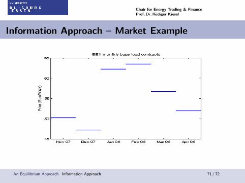
Market Risk Premium – Information Approach
Since electricity is non-storable future predictions about themarket will not affect the current spot price, but will affectforward prices.Stylized example: planned outage of a power plant in onemonthMarket example: in 2007 the market knew that in 2008 CO2emission costs will be introduced; this had a clearly observableeffect on the forward prices!
An Equilibrium Approach Information Approach 70 / 72
Chair for Energy Trading & FinanceProf. Dr. Rüdiger Kiesel
Information Approach – Market Example
Introduction The spot-forward relation The information approach The equilibrium approach Conclusions
An Equilibrium Approach Information Approach 71 / 72
Chair for Energy Trading & FinanceProf. Dr. Rüdiger Kiesel
Information Approach – Definition
Define the forward price as
FG(t,T ) = E[S(T )|Gt ]
Gt includes spot information up to current time (Ft) andforward looking informationThe information premium is
lG(t,T ) = FG(t,T )− E[S(T )|Ft ].
Theoretical analysis uses the theory of enlargements offiltrations
An Equilibrium Approach Information Approach 72 / 72