THE DEVELOPMENT OF THE ONTARIO HIGHWAY BRIDGE DESIGN CODE

P.F. Csagoly and R.A. Dorton, Ontario Ministry of Transportation and Conununications

At the end of 1975, the Ontario Ministry of Transportation and Conununications decided to develop a Code for designing Ontario's highway bridges. Structural research in the Ministry, which began in 1969, has been successful in clarifying several aspects of structural behavior and load-carrying capacity. The activities concentrated on proof-testing exist­ing bridges of questionable strength, inspecting and recording a large number of structures for various conunon faults; many the result of inadequate design practices. The resulting Ontario Highway Bridge Design Code is based on the existing AASHTO Specifications, but with most provisions for working stress design eliminated. For both serviceability and ultimate limit states, an upper-bound representation of all commercial vehicles observed in Ontario through various load surveys is employed. The use of deflection and stiffness criteria has been re-evaluated for each structural material. Impact and dynamic response is treated as a function of resonance frequencies. While introducing provisions for 0.3% deck reinforce­ment, crack control is made mandatory. The Code will discourage the use of single load path structures. New provisions on hydrology, drainage and various dimensional requirements are intended to achieve low maintenance structures. New sections are devoted to non­traditional analysis, soil-steel structures and the evaluation of existing bridges.

The objective of this paper is to highlight the new provisions of the Code and to provide information on the background research and study which led to their inclusion.

Background Research and Testing

In 1966 the Ontario Trucking Association made several presentations with the aim to increase the permissible weight of commercial vehicles. Although the legal Ontario weights were nearly twice as large as those recommended by AASHTO CJ), the Ontario highway bridges had shown no distress due to overloading. This created skepticism of the validity of the AASHTO Code. The Ministry responded

to this skepticism and originated a bridge testing program in 1969, in order to identify the magnitude of extra load-carrying capacity hidden due to the suspected conservatism of the Specifications and the unrefined nature of "traditional" methods of structural analysis.

The testing program, which at the time of writing this paper included over 125 bridges, revealed three significant facts:

1. The actual load-carrying capacity of highway bridges can exceed by a substantial margin the value established by "traditional" methods of analysis.

2. The load-carrying capacity can be predicted with certainty by refined methods of analysis, verified in turn by prototype bridge testing.

3. The margin of unaccounted-for extra capacity was observed to vary between 10% on steel trusses to 3,000% on concrete rigid frames.

Rationale for a New Code

It was considered important to have available a metric design code in 1978, as this is the target date for metric conversion for the construction industry in Canada. The most important factor in the Ministry's final decision to write a new Code was the availability of several significant research and development findings from Ministry work carried out by universities and the Ministry's Research and Development Division. Documentation more substantial than internal research reports was required as bridge designers need the backing of an accepted specification for their regular design activities, and it was thus essential to codify the research findings. The time necessary to incorporate these into either the CSA (~) or AASHTO (l) codes was considered prohibitive. In addition, the uncertainty in these specifications over the use of load factor or limit states design did not coincide with the Ministry's objectives to have a rational limit states format in operation as soon as possible to the exclusion of all other methods.

Preparation of the Code

The task force comprising 95 engineers is governed by an 11 member Code Control Conunittee,

l

2

which is responsible for the general concepts and broad philosophy of the Code as well as the review and acceptance of the technical sections written by sub-committees. The Code Control Committee is represented by MTC, the federal government of Canada, universities, and consulting engineers.

A sub-committee was formed for each of the 17 anticipated Code Sections, with chairmen appointed from MTC or the universities. The average committee size is five, and the sub-committee membership is from governments, universities, consulting engineers and industry of Canada and the United States.

Writing of the Code was begun immediately following a seminar in May 1976, attended by all members. Following reviews of content and outline, the first drafts were submitted in March 1977. These were subjected to detailed review by the Code Control Committee and revised drafts were submitted for editing. These edited drafts were issued for public comment in February 1978 with the final content of the Code scheduled to be completed late in 1978.

Each Section of the Code will consist of four possible subdivisions:

1. The Code proper which will be prescriptive and binding.

2. Charts or diagrams giving detailed data in an Appendix which will be binding.

3. A commentary giving justification or background information on each Code clause.

4. A supplement of background data or research information considered essential for a full under­standing of the Code.

General Concepts

The first proposal for a new design load based on survey data on actual truck loadings in Ontario was given in 1973 (1). In addition to the live loading model it defined a load factor approach and a new proposal for dynamics of bridges.

The most important concept established for the Code was that it should be presented in the Limit States format. This was to apply to all Sections and all materials, and meant that the Working Stress method of the present CSA-S6 and the optional Working Stress or Load Factor approach of AASHTO would not be permitted. The Limit States approach requires that load factor and performance factor values be given in the Code, based on statistical data on load and strength variations, and calibrated to a pre-selected value for the Safety Index 13.

A major objective of the Code was to transfer the growing knowledeP of thP. Hf'_t:uBl behavior of existing bridges from the full-scale load test program (4, 5, 6) into definable clauses for the evaluatio~ of the load-carrying capacity of existing bridges. In addition to evaluation methods based on testing experience, the Code defines rating and posting loads that are directly related to the design loads for new bridges and hence the existing trucks on the highway. The increased concern for minimizing maintenance is expressed through new clauses covering bridge hydraulics, deck drainage and durability.

The importance of advanced techniques is evidenced by the addition of a Section on "Methods of Analysis" which gives guidance on analytical methods that are accepted or recommended. The Code is a design code, and hence construction items have only been included if they were considered essential to the designer.

Limit States Design

Background

Limit States Design was developed and adopted for structural design during the 1950s, and has since been widely accepted by many European countries. General use of the method in North America has been somewhat slower, although the basis was established as early as 1963 in the ACI Building Code (]_),but under different terminology.

The advantages of the Limit States Design approach towards achieving more uniform structural safety and economy are well documented (9, 10, 11). Safety and Limit States Design are compr-;hensively defined by MacGregor (9) and were used extensively in the development of the Code. He states: "When a structure or structural element becomes unfit for its intended use it is said to have reached a limit state.

Limit States Design is a design process that involves:

1. Identification of all potential modes of failure, i.e. limit states.

2. Determination of acceptable levels of safety against occurrence of each limit state.

3. Consideration by the designer of the sig­nificant Limit States."

The Code defines the Limit States in two groups, Ultimate Limit States and Serviceability Limit States (~).

Ultimate Limit States

The ultimate limit states correspond to the maximum load-carrying capacity of the bridge or a component, and are associated with the extreme loading cases. These states may result from loss of equilibrium, fracture of a section, formation of a mechanism due to plastic hinge development, and buckling.

Elastic methods of analysis are to be used in determining the response of the structure at the ultimate limit states, which is consistent with current North American codes such as AASHTO (1), NBC (7), and ACI (12), and most European code-;;-, While-it is true that the structure is unlikely to behave elastically throughout the load range, and that plastic redistribution will occur normally before an ultimate limit state is reached, it is recognized that methods of analysis involving inelastic behavior are not generally available to the designer at present.

The ultimate strength calculation of sections is based on the present well-established North American procedures. For reinforced concrete in flexure the calculation is based upon strain compatibility and an equivalent rectangular concrete stress distribution at the 0.85 f~ level. For steel sections in flexure, the plastic moment is assumed to be attained for braced compact sections, but the yield moment is used for non-compact and unbraced sections.

For the ultimate limit state design calculations, load factors are applied to all load and force effects, and performance factors to the resistance or strength.

Serviceability Limit States

The serviceability limit states concern the disruption of the functional use of the structure

and are associated with the loadings for normal use. A bridge may be considered to have reached the serviceability limit state because of local damage such as cracking and spalling of concrete, vibration, excessive deflection, and fatigue. Elastic methods of analysis should be used to determine the response, as the structure is expected to behave elastically at the stress level or deflection value specified for these states.

There are two live load levels to be considered for the serviceability limit states. For fatigue, where the accumulation of many repeated events is the criterion, the live load corresponds to one heavy truck train. This service load is also applied to vibration calculations for human response. A multiple truck loading must be considered for states such as local damage and permanent defor­mation below the ultimate level.

Some serviceability limit states were covered implicitly in the Working Stress Methods of previous codes. They are now more clearly defined, the loadings and checks are more explicit, and many are new to bridge codes.

Human response to vibration, for bridges designed for varying pedestrian use, is covered by a frequency dependent limit on dynamic deflection. For substructure design, settlement is the most important serviceability condition, as any differ­ential settlement causes superstructure and roadway deformations.

The cracking level of deck slabs is a critical criterion for deck durability. Cracking in all reinforced concrete is controlled by a service level limit on tensile reinforcement stresses, with the value dependent upon exposure conditions.

For steel the live load deflection limitations of previous codes have been removed, to be replaced by new dynamic and vibration controls. Inelastic deformation must not take place at the serviceability limit state to prevent permanent set. For high strength friction bolts in shear, the slip of the connected parts is controlled. Fatigue limits are set as a service condition for main members, connections and secondary members in steel.

For bearings and expansion joints, performance under the movements due to temperature, shrinkage, creep, and live load is a service level condition.

The serviceability limit state conditions are many and varied, and each designer will have to ensure that all the states appropriate to the particular structure being designed are properly investigated.

Design Equation

For the ultimate limit state the required design relationship is that the factored resistance must exceed the sum of the factored load effects. Thus:

cj>R ;;., l: KL

where:

cp = Performance Factor R K L

Resistance Load Factor Load Effect

The performance factor cJ> is applied to the resistance to account for the variabilities in material properties, dimensions and workmanship,

(1)

the uncertainties in methods of computing resistance, and the type of failure being avoided. The load factors K are applied to the loads to account for

3

uncertainties in the analytical methods, the unpre­dictable behavior of the structural system and to account for the variability of the loads themselves.

As the variability in loads would be expected to be non-uniform among dead load, live load and earth pressure, for instance, different values of K could be expected. Similarly the variability in dimensional tolerances between steel beams, cast-in­place concrete and asphalt, for instance, would indicate the same. For simplicity, AASHTO has used a value of K = 1.3 for all loads, and varied the live load magnitude for different load combinations.

In the Ontario Code greater precision has been sought by selecting the best value for the load factor for live load and each of four different dead load effects. The extra work involved in using a number of lo.ad factors is justified by the improved accuracy. This is particularly true as spans increase and the variable dead load factors produce a significant improvement in accuracy, and hence in more uniform safety and economy.

Th~ separation of cp and K factors has been maintained throughout the Code. This should be borne in mind if a comparison is made with AASHTO, where separation has been maintained for reinforced concrete, but only load factors are given for steel, without performance factors. In actual fact, the load factor given for steel is a combination of both factors, or K/cj>, but quoted as a load factor (13).

The values of K and cJ> used in the Code we~ derived as part of the Code calibration process described later.

Design Live Load

That the bridge design live load vehicle should be directly related to the legal highway vehicle appears self-evident. The fact that this relationship is very difficult to discern in many jurisdictions is, however, true. This is probably due to the fact that authors of bridge codes are not usually in a position to set or administer legal truck weights.

The maximum legal weights in 1944 were similar to the 320 kN (72 kip) AASHTO Standard HS 20 truck which was first specified for bridge design in that year. This loading is still conunonly accepted in North America, except for those who specify an HS 25 truck. Since 1944 the legal weights have increased substantially reaching a peak value of 623 kN (140 kips) in Ontario.

Maximum Truck Weights

Ontario's present maximum legal weights for trucks were established in 1971 following extensive study of the effects of the proposed increases upon bridge response (!~_). The formula which determines the allowable gross weight, axle weights, or combinations of axles is known as the Ontario Bridge Formula (OBF). It relates the allowable weight W in kips to the equivalent base length BM in feet, in the following manner.

w 20 + 2.07BM - 0.0071B~

The equivalent base length is defined as the length over which the total weight on a group of axles should be uniformly distributed in order to produce substantially the same response on a bridge as the group of axles itself. BM is calcu­lated by an equation whose inputs are individual axle weights and interaxle spacings. With this

(2)

4

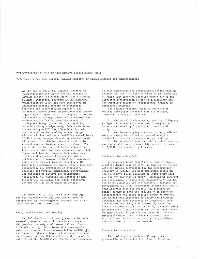
transformation any vehicle or group of axles can be quickly evaluated for acceptability. The formula has been plotted as the lower curve in Figure 1. The two limits are W = 89 kN (20 kips) when BM = 0, which is the single axle case, and W = 623 kN (140 kips) when BM= 24.4 m (80 ft.), which is the maximum BM value that can be generated with a legal vehicle length limit of 19.8 m (65 ft.). The various axle groups for the HS 20 truck have been plottPn on this diagram, and it can be seen that this live load model represents only the lower part of the legal weight curve (OBF).

The legal weight curve can only act as the basis for a design live load if actual weights never exceed the legal weights, which implies perfect enforcement with no tolerance. To ascertain actual truck weights, major surveys have been carried out at truck inspection stations in Ontario. A survey of 7,292 vehicles was taken in 1971 and results were plotted to compare with the legal weight curve. The first effort to establish a bridge design load based on this survey data was made in 1973 (3), using an upper-bound weight curve known as the-Maximum Observed Load (MOL) curve. This upper bound was best represented by a curve with a constant band width of 100 kN (22.5 kips) above the legal weight curve (OBF), as shown in Figure 1.

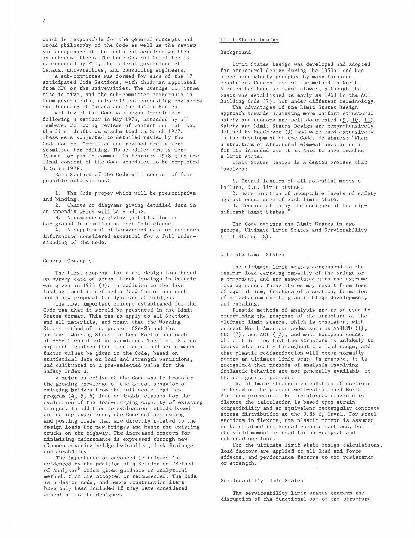
To verify the actual weights surveyed in 1971, another survey of 9,864 vehicles, preselected to be representative of the heavy trucks, was carried out in 1975. It was found that the MOL was still a satisfactory upper-bound curve, but the percentage of trucks falling between the OBF and MOL curves had increased since 1971. In 1978, improved weight enforcement procedures were introduced. The new regulations are based on a modified Bridge Formula in SI units shown in Figure 2. The corresponding modified MOL level was adopted as the basis for a design live load model.

Live Load Design Models

A live load design system must model the following two aspects:

1. One heavy vehicle. This should incorporate the effect of axle loadings for the design of the floor system and short span members. The single vehicle itself will also govern the design of short to intermediate span bridges.

2. The presence of several vehicles. There are two components of multiple presence. First, the presence of more than one vehicle in a lane, and second, the presence of vehicles in more than one lane. The first component applies to bridges above the short span range, and most continuous structures. The second affects all multi-lane structures.

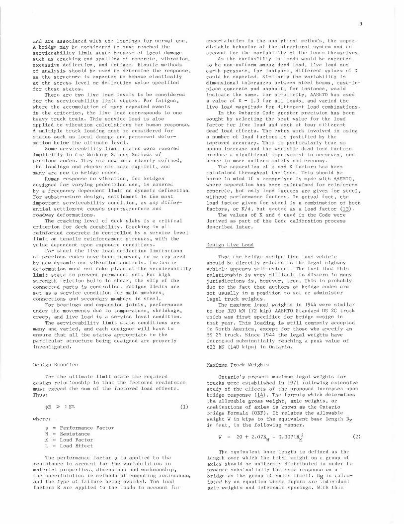
The single heavy vehicle model should be an upper-bound representation of all vehicle weights, as it will be applied to a design for the ultimate limit state. The MOL curve was used as the basis for developing the truck model which has to produce the maximum response for both moment and shear using either the whole truck or individual axles or axle combinations. No single actual truck from the surveys could produce this required response, and hence an idealized 5-axle vehicle was developed (Figure 3) which is ref erred to as the OHBD truck and rese bles a real truck configuration. The plot of this OHBD truck and four other axle groupings thereof, using the BM transformation compared to the MOL curve (Figure 2), shows its suitability for capturing maximum responses.

Figure 1. Ontario Bridge Formula (OBF) curve .

160

140

120

JOO

80

en ~ 60 :.'.

~ HS20 TRU CK ;;: 40 B 32 32 KIPS

...: r 1 * ;;: ' _1_2 __ 3

I

en 20 I~ en ' 4 I 0 a:: (!)

0 20 40 60 00 EQUIVALENT BASE LENGTH, BM IN FEET

Note: 1 kN = 0.225 kip 1 m = 3.28 ft .

Figure 2. Maximum Observed Load (MOL) curve.

600

700

600

Q. ~

5 ~

"' 400 OHBO TRUCK ...J x 60 140l40 200 ..

j 11 l i!i ....

~ .....!..... i3 w ~ ;i 4 ...J ~ 5 g 6

7

0 10 16 20 25

EQUIVALENT BASE LENGTH, Bm

Note : 1 kN = 0.225 kip 1 m = 3.28 ft.

160 kN

I

30 (111 )

Figure 3. Diagram of Ontario Code design truck.

60 140140 200 160 AXLE LOAD

l l~ l ~ IN kN

GROSS WT.

I: ... ~. .I. j =700 kN

G.O 7.2

18m

OHBD TRUCK Note: 1 kN = 0.225 kip

1 m = 3.28 ft.

Determining the suitability of this OHBD truck for the wide variety of continuous structures in use, and developing the multiple presence aspects of a live load system required a large statistical study (_!2). A statistical description of Ontario truck traffic was developed which included the following:

1. 6,825 trucks taken from the 1975 survey. 2. A probability distribution of gross weight

ratio, which is the ratio of gross truck weight to the legal weight li~it, based on the 1975 survey.

3. A probability distribution for headway distance between trucks.

The Code's sub-committee responsible for the live load system selected the 700 kN (157.5 kip) OHBD truck as the idealization of one heavy vehicle. This decision was based on the truck's ability to best capture various responses based on the MOL study and the University of Western Ontario report (_!2), and the fact that it was the simplest and most practical model.

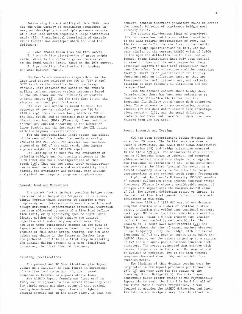
The live load system selected to model the presence of several vehicles uses one 490 kN (110.2 kip) truck in each lane, which is 70% of the OHBD truck, and is combined with a uniformly distributed load (UDL) (Figure 4). Lane reduction factors are applied according to the number of lanes loaded, and the intensity of the UDL varies with the highway classification.

For the serviceability limit states the effect of the mean of the loaded frequently occurring vehicles was required. The service load has been selected as 80% of the OHBD truck, thus having a gross weight of 560 kN (126 kips).

The loading to be used for the evaluation of existing bridges and for posting purposes is the OHBD truck and two subconfigurations of this truck (.1§). Thus the one basic truck configuration can be used for ultimate and serviceability limit states, for evaluation and posting, with obvious analytical and computer programming advantages.

Dynamic Load and Vibrations

The impact factor in North American bridge codes has remained unchanged for 50 years. It is a very simple formula which attempts to describe a very complex dynamic interaction between the vehicle and bridge structure. Objectionable structural vibration has been addressed by means of a live load deflec­tion limit, or by specifying span to depth ratio limits, neither of which achieve the desired objective with modern highway structures. The new Code makes substantial changes in the area of impact and dynamic response based primarily on the results of full-scale bridge testing. The new Code values may change in the future as further data are gathered, but this is a first step in relating the dynamic design process to a more significant parameter, the first flexural frequency.

Existing Specifications

The present AASHTO Specifications give impact values as a function of span length in percentage of the live load to be applied, i.e. dynamic response is treated as a quasi-static load.

The AASHTO impact formula was first used in 1927, and it appears to have served reasonably well for simple spans and short spans of that period, having been based on impact tests of highway bridges carried out in the early 1920s. It does not,

5

however, contain important parameters found to affect the dynamic behavior of continuous bridges more recently built.

The current slenderness limit of span/depth <25 for beams has had its evolution traced back to the AREA railway specification of 1905. The limitation on deflection was first introduced in railway bridge specifications in 1871, and was very similar to the current AASHTO value of 1/800 of the span for deflection due to live load and impact. These limitations have only been applied to steel bridges and the sole reason for their retention appears to have been expectation that user discomfort from vibrations would be controlled thereby. There is no justification for keeping these controls on deflection today as they are inadequate for their intended use, and criteria relating to user response to vibrations can now be specified.

With the present concern about bridge deck deterioration there has been some reluctance to abandon the deflection limits for fear that increased flexibility would hasten deck deteriora­tion. There appears to be no correlation between flexibility and deck deterioration from investiga­tions reported (.lZ) , and the usual deflection controls for steel and concrete bridges have been deleted from the new Code.

Recent Research and Testing

MTC has been investigating bridge dynamics for more than 20 years. The initial work was done at Queen's University, and dealt with human sensitivity to vibration (ll) and bridge vibrations measured in the field (!2_,_.?.Q). The measurements were carried out on 52 bridges known to vibrate, and recorded mid-span deflections with a simple deflectograph. The frequency of vibration of the loaded structures was generally the first flexural frequency, or a forced frequency usually in the 2 to 7 Hz range, corresponding to the typical truck bounce frequencies.

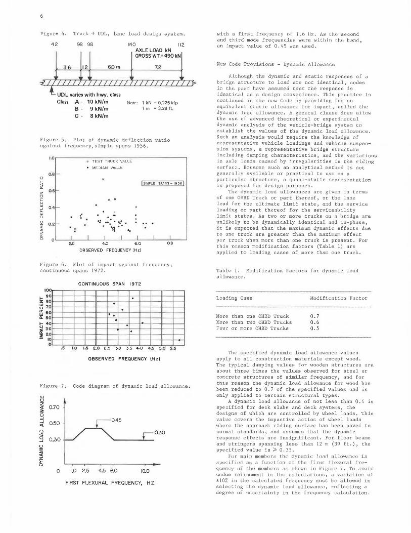
A plot of the Queen's University 1956-57 results of dynamic deflection ratio against observed bridge frequency (Figure 5) shows a considerable number of bridges with impact over the maximum AASHTO value of 0.3. The dynamic deflection ratio, or impact, is the ratio of live load dynamic deflection to static deflection at mid-span.

Between 1969 and 1971 MTC carried out dynamic response studies on a number of continuous struc­tures, including the voided post-tensioned concrete deck type. MTC's own load test vehicle was used for these tests, being a 5-axle tractor semi-trailer unit with load varied by concrete blocks. The results of 11 tests have been reported (21) and Figure 6 shows the plot of impact agains--;:-observed bridge frequency. Only one bridge, with a flexural frequency of 5.8 Hz, gave an impact value below the AASHTO figure, and the values ranged up to a maximum of 87% for a 5-span, post-tensioned concrete deck structure. The report suggested that bridges with natural frequencies in the 2 to 5 Hz range should be avoided if possible, due to the high dynamic response observed when bridge and vehicle f re­quencies match.

The findings of this dynamic testing were in­corporated in the impact proposals put forward in 1973 (]) and were used for the design of the Conestoga River Bridge (4,5). For this 3-span continuous plate girder bridge it was economically impossible to avoid the 2 to 5 Hz band t'or all of the first three flexural frequencies. It was decided to abandon the AASHTO deflection and depth limitations and design a very flexible structure

6

Figure 4. Truck -I UDL, laue luatl ui=slgu systt:m.

42 98 98 140 112 AXLE LOAD kN GROSS WT.=490 kN

.G L2 6.0 m

UDL varies with hwy. class

Class A - 10 kN/m B 9 kN/m C - 8 kN/m

72

Note: 1 kN = 0.225 kip 1 m = 3.28 ft.

Figure 5. Plot of dynamic deflection ratio against frequency, simple spans 1956.

i.o TEST TRUCK VALUE • . MEDIAN VALUE

0.8 0 j:: I SIMPLE SPANS - 1956 I <t a: z Q.6 0 j:: . a u w 0 .4 --' "-w -: 0

•: . u 0 .2 .. 0 • ~: •

:E 'i -<t .. z >-0 0

2.0 4.0 6 .0 0.8

OBSERVED FREQUENCY (Hz)

Figure 6. Plot of impact against frequency, continuous span s 1972.

CONTINUOUS SPAN 1972

f-- 90 2: 80 w 70 u a: 8 0 L&J .. a.. !1 0 f-- 401 1-~1--~1--~-1-~t-~+-~-1---,;1~-1.a..-1-~f--~I--_..,

~ 3 011--~f--~f---t~--1-~-t-~-r-~-1-~+-~!--~l-~f----l ~ 20f---l~-11--~1--<f----<~-1~--1~-t~-+~--1~-1~--1 - 101--~1--~1--~1--~1--~~-1~--1~-t~-1-·--tf--~1--...-i

C'----.i,~_._......,~--::1-:--::-1=---,:L----''---'-~.,.L,----,!L,,--........L,,..-~ .5 1.0 1.11 2 .0 2 .5 3.0 3 .5 4 .0 4.5 s.o 5 .:1

OBSERVED FREQUENCY {Hz)

Figure 7. Code diagram of dynamic load allowance .

w u z <( ~

0.70

0 ....I 0 .45 ....I 0.50 <(

0 0.30 <(

g 0.30 u ~ <( z 6

0 1.0 2.5 4.5 6.0 10.0

FIRST FLEXURAL FREQUENCY, HZ

wich a first f r e quency of i.b Hz. As the second and third mode fr e quencies were within the band, an impact value of 0.45 was us e d.

New Code Provisions - Dynamic Allowance

Although the dynamic and static responses of a bridge structure to load are not identical, codes in the past have assumed that the response is identical as a design conveni ence . This practice is continued in the new Code by providing for an e quivalent static allowance for impact, called the dynamic loa<l allowance. A general clause does allow the use of advanced theoretical or experimental dynamic analysis of the vehicle-bridge system to establish the val ues of the dynamic load allowance. Such an analysi s would require the knowledge of representative vehicle loadings and vehicle suspen­sion systems, a representative bridge structure including damping characteristics, and the variations in axle loads caused by irregularities in the riding surface. Because such an analytical method is not generally available or practical to use on a particular structure, a quasi-static representation is proposed for design purposes.

The dynamic load allowances are given in terms of one OHBD Truck or part there of, or the lane load for the ultimate limit state, and the service loading or part thereof for the serviceability limit states. As two or more trucks on a bridge are unlikely to be dynamically identical and in-phase, it is expected that the maximum dynamic effects due to one truck are greater than the maximum effect per truck when more than one truck is present. For this reason modification factors (Tab l e 1) are applied to loading cases of more than one truck .

Table 1. Modification f ac t ors for dynamic l oad al l owance .

Loading Case

More than one OHBD Tru ck More than t wo OHBD Truck s Four or more OHBD Tru cks

Modification Factor

0.7 0 . 6 0 . 5

The specifie d dynamic load allowance value s apply to all construction materials except wood. The typical damping VQ.lues for wooden structures are about three times the values observed for steel or concrete structures of similar frequency, and for this reason the dynamic load allowance for wood has been reduced to 0.7 of the specified values and is only applied to certain structural types.

A dynamic load allowance of not less than 0.4 is specified for deck slabs and deck systems, the designs of which are controlled by wheel loads. This value covers the impactive action of wheel loads where the approach riding surface has been paved to normal standards, and assumes that the dynamic response effects are insignificant. For floor beams and stringers spanning less than 12 m (39 ft.), the specif ied value is~ 0 . 35.

For main memb ers the dynami c load allowance is specified as a function of the first flexural fre­quency of the members as shown in Figure 7 . To avoid undue refinement in the calculations, a variation of ±10% in the calculated frequency must be allowed in s e le cting the dynamic load allowance, reflect i ng a degree of uncer t ainty in the frequency calculation .

For flexible, long-span structures with a fre­quency of less than 1 Hz, and short-span structures with a frequency greater than 6 Hz, the maximum AASHTO impact value of 0.3 is retained for the dynamic load allowance. For structures where a resonance condition is possible, values are reaching a maximum value of 0.45 in the band of 2.5 Hz to 4.5 Hz. The pitch and bounce frequencies of most heavy commercial vehicles in Ontario fall within this band.

New Code Provisions - Vibration Control

A serviceability limit state has been specified to control objectionable vibrations for pedestrian users of various types of bridges. To achieve this control, a restriction has been placed on deflection in relation to the first flexural frequency of the bridge.

Structures have been placed in four classes, each class having its own deflection-frequency limit curve. These curves have been based on a number of studies of human response to vertical vibration (~,11_), with the acceleration parameter changed to the equivalent deflection parameter for ease of calculation.

Methods of Analysis

The present AASHTO Specifications give little guidance on methods of static analysis for bridge superstructures, except for the clauses on distribution of loads. In the new Ontario Code, the section on methods of analysis replaces the load distribution clauses and expands the coverage to indicate approved methods of design analysis.

Background

It has long been recognized that the distribu­tion factors given in AASHTO are lower-bound values to cover a wide variety of cases, and thus lead to overdesign for some structures. There has always been a general clause which allows a rational analysis to replace an empirical formula, but there has been little active encouragement to use advanced methods of analysis.

The removal of the deflection limitation for steel beams could lead to more flexible structures, for which the load distribution is better than for present structures. As an example, the Conestoga River Bridge (4) had an equivalent distribution factor of S/7.S based on a grid analysis, compared to the AASHTO empirical value of S/5.5. While the simple distribution factor approach has served well in the past, and was necessary when more complex analysis was very time-consuming, the availability of computer programs for advanced methods of analysis means the empirical approach is not appro­priate for all structures today.

For these reasons the distribution factor approach has been reconsidered, and where still found acceptable, has been given in a more accurate format, but much of the simplicity of the old method has been retained. For the areas considered un­acceptable, preferred methods of refined analysis are given for different categories of structures. In addition, guidanc2 is given on conditions affecting the selection of the method of analysis and on the idealization of structures for analysis.

Simplified Methods

Two simplified methods of analysis are allowed, subject to prescribed conditions being fulfilled. One is a distribution coefficient method and the other is the beam analogy method.

7

The distribution coefficient method is comparable to the AASHTO distribution factor method, the application being similar by the use of a load fraction S/D applied to the wheel loads. D is given a value in AASHTO according to bridge type, but is selected from charts for each bridge by the Ontario Code in accordance with the number of lanes and the stiffness properties of the particular structure, thus providing improved accuracy. The method is approved for use in calculating longitudinal moments and shears in bridges with shallow superstructures, subject to restrictions on continuity, skew, curva­ture, beam spacing, and variations in section. The shallow superstructures to which the method applies include solid slabs, shallow voided slabs, slabs on girders, grillages and shear connected beams.

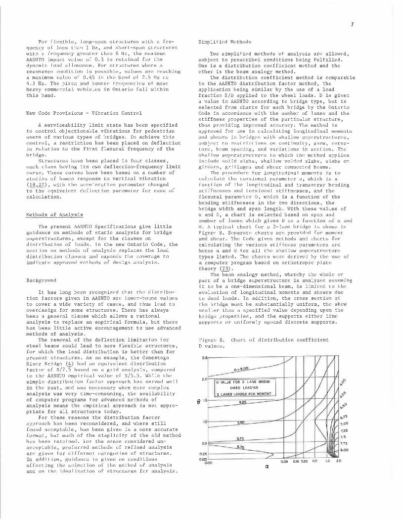
The procedure for longitudinal moments is to calculate the torsional parameter a, which is a function of the longitudinal and transverse bending stiffnesses and torsional stiffnesses, and the flexural parameter 8, which is a function of the bending stiffnesses in the two directions, the bridge width and span length. With these values of a and 8, a chart is selected based on span and number of lanes which gives D as a function of a and 8. A typical chart for a 2-lane bridge is shown in Figure 8. Separate charts are provided for moment and shear. The Code gives methods and charts for calculating the various stiffness parameters and hence a and 8 for all the shallow superstructure types listed. The charts were derived by the use of a computer program based on orthotropic plate theory (23).

The beam analogy method, whereby the whole or part of a bridge superstructure is analyzed assuming it to be a one-dimensional beam, is limited to the evaluation of longitudinal moments and shears due to dead loads. In addition, the cross section of the bridge must be substantially uniform, the skew smaller than a specified value depending upon the bridge properties, and the supports either line supports or uniformly spaced discrete supports.

Figure 8. Chart of distribution coefficient D values .

1.0

a

00 ro·

.,'Y"'

.,~o

o:r~

,,oo

7.Z5

7,5

7.75

e.oo

2.0

8

Refined Methods

The following methods are approved for general use for the analyses of the appropriate bridge types :

1. Grillage analogy methods. 2. Orthotropic plate theory methods. 3. Finite element methods. 4. Finite strip methods. 5. Folded plate methods.

These refined methods are well reported in the technical literature and the Code gives referenc e to representative pape rs without further detailing of the methods. The Code doe s, however, give detailed guidance on the idealization of shallow structures for analysis by both 2-dimensional and 3-dimensional anal ytical methods.

Selection of Methods of Analysis

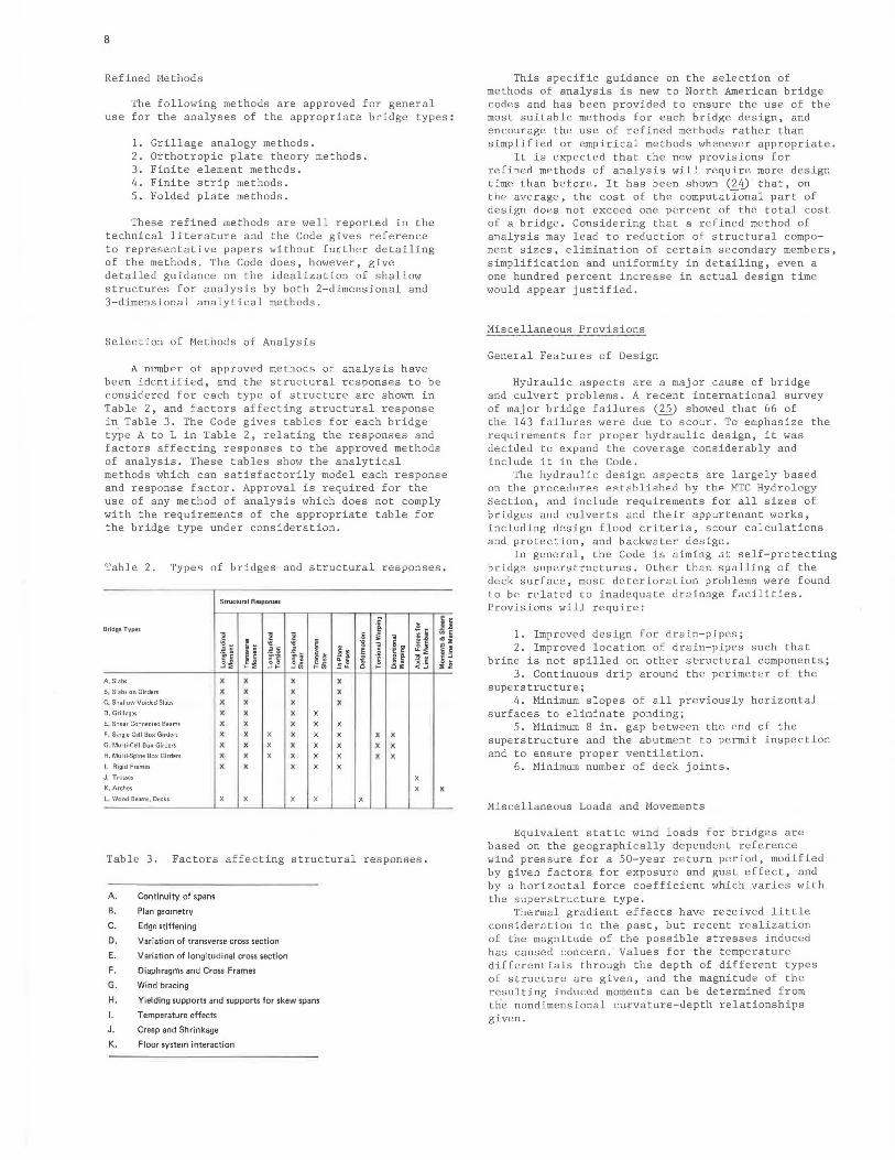
A number of approved methods of analysis have been identified, and the structural responses to be c onsidered for each type of structure are shown in Table 2, and factors affe c ting structural response i n Table 3. The Code gives tables for each bridge type A to Lin Table 2, r e lating the responses and factors affecting response s to the approved methods of analysis. These tables show the analytical methods which can satisfactorily model each response and response factor. Approval is required for the use of any method of analysis which does not comply with the requirements of the appropriate table for the bridge type under c onsideration.

Table 2 . Types of bridges and structural responses.

Structural Responses

BridQ8 Types ·~ ~ i j iij &£

A, Slabs

B, Slabs on Girders

C. Shallow Voided Slabs

O.Grillages

E. Shear Connected Beams

F, Single Cell Box Girders

G. Multi Cell Box Girders

H. Multi·Spine Box Girders

I Rigid Frames

J, Trusses

K. Arches

L, Wood Beams, Decks

x

x x

x

~ 2 ~. t~ l H ti g _,,_ _,.:;

x x x x x x x

x x x

x

c ~ j ~ ~ 0

·~ ~ ~ £ . " ~ I · ~ t: ·=· ~" ~ ~ " ~ ~ ~ ~ ·~ .~ ,_.:; ~if 0 (:. o~ < _,

x x x

x x x x x x x x x x

x x

Table 3. Factors affe c ting structural responses.

A. Continuity of spans

B. Plan geometry

C. Edge stiffening

D. Variation of transverse cross section

E. Variation of longitudinal cross section

F. Diaphragms and Cross Frames

G. Wind bracing

H. Yielding supports and supports for skew spans

I.

J .

Temperature effects

Creep and Shrinkage

K. Fl9or system interaction

'" :o t~ r ~

x

This specific guidance on the selection of methods of analysis is new to North American bridge codes and has been provided to e.nsure the use of the most suitable methods for each bridge design, and encourage the use of refined methods rather than simplified or empirical methods whenever appropriate.

It is expected that the new provisions for refined methods of analysis will require more design time than before. It has been shown (24). that, on the average, the cost of the computational part of design does not exceed one percent of the total cost of a bridge. Considering that a refined method of analysis may lead to reduction of structural comp o­nent sizes, elimina t i on of certain secondary members, simplification and uniformity in detailing, even a one hundred percent increas e in actual design time would appear justifie d.

Miscellaneous Provisions

General Features of Design

Hydraulic aspects are a major cause of bridge and culvert problems. A recent international survey of major bridge failures (25) showed that 66 of the 143 failures were duet;;' scour. To emphasize the requirements for proper hydraulic design, it was decided to expand the cove rage considerably and include it in the Code.

The hydrauli c design aspects are largely based nn the proc-eduries est abli s hed by thie MTC Hydro logy Section, and include requirements for all sizes of bridges and culverts and their appurtenant works, including design flood crite ria, scour calculations and protection, and backwater design.

In general, the Code is aiming at self-protecting bridge superstructure s. Other than spalling of the deck surface, most d e terioration problems were found to be related to inadequate drainage facilities. Provisions will requi re:

1. Improved design for drain-pipes; 2. Improved location of drain-pipes such that

brine is not spilled on other s~ructural components; 3. Continuous drip around the perimeter of the

superstructure; 4. Minimum slopes of all previously horizontal

surfaces to eliminate ponding; 5. Minimum 8 in. gap between the end of the

superstructure and the abutment to permit inspe c tion and to ensure proper ventilation.

6. Minimum number of deck joints.

Miscellaneous Loads and Movements

Equivalent static wind loads for bridges are based on the geographi c ally dependent reference wind pressure for a 50-year return period, modified by given factors for exposure and gust effect, and by a horizontal force coefficient which varies with the superstructure type.

Thermal gradient effects have received little consideration in the past, but recent realization of the magnitude of the possible stresses induced has caused concern. Values for the temperature differentials through the depth of different types of structure are given, and the magnitude of the resulting induced moments can be determined from the nondimensional c urvature-depth relationships given.

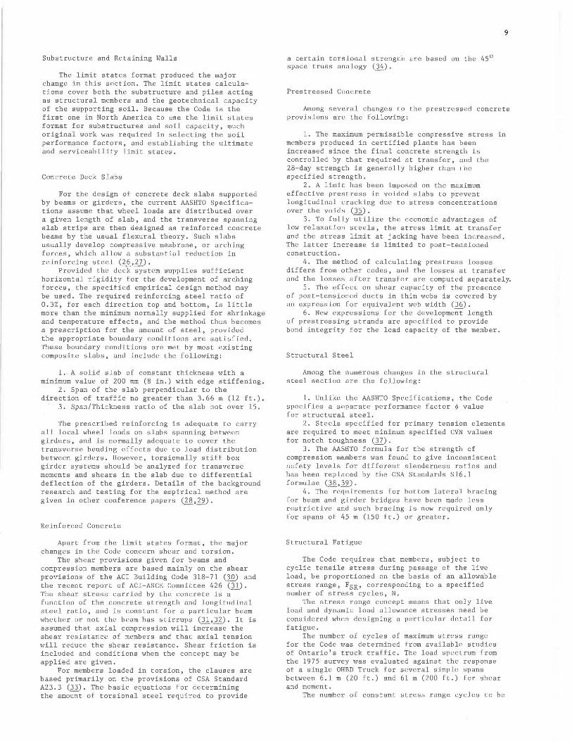
Substructure and Retaining Walls

The limit states format produced the major change in this section. The limit states calcula­tions cover both the substructure and piles acting as structural members and the geotechnical capacity of the supporting soil. Because the Code is the first one in North America to use the limit states format for substructures and soil capacity, much original work was required in selecting the soil performance factors, and establishing the ultimate and serviceability limit states.

Concrete Deck Slabs

For the design of concrete deck slabs supported by beams or girders, the current AASHTO Specifica­tions assume that wheel loads are distributed over a given length of slab, and the transverse spanning slab strips are then designed as reinforced concrete beams by the usual flexural theory. Such slabs usually develop compressive membrane, or arching forces, which allow a substantial reduction in reinforcing steel (±2_,1]_).

Provided the deck system supplies sufficient horizontal rigidity for the development of arching forces, the specified empirical design method may be used. The required reinforcing steel ratio of 0.3%, for each direction top and bottom, is little more than the minimum normally supplied for shrinkage and temperature effects, and the method thus becomes a prescription for the amount of steel, provided the appropriate boundary conditions are satisfied. These boundary conditions are met by most existing composite slabs, and include the following:

1. A solid slab of constant thickness with a minimum value of 200 mm (8 in.) with edge stiffening .

2. Span of the slab perpendicular to the directio.n of traffic no greater than 3.66 m (12 ft.) .

3. Span/Thickness ratio of the slab not over 15.

The prescribed reinforcing is adequate to carry all local wheel loads on slabs spanning between girders, and is normally adequate to cover the transverse bending effects due to load distribution between girders. However, torsionally stiff box girder systems should be analyzed for transverse moments and shears in the slab due to differential deflection of the girders. Details of the background research and testing for the empirical method are given in other conference papers (~,12_).

Reinforced Concrete

Apart from the limit states format, the major changes in the Code concern shear and torsion.

The shear provisions given for beams and compression members are based mainly on the shear provisions of the ACI Building Code 318-71 (30) and the recent report of ACI-ASCE Committee 426 (31). The shear stress carried by the concrete is a function of the concrete strength and longitudinal steel ratio, and is constant for a particular beam whether or not the beam has stirrups (11.,21_). It is assumed that axial compression will increase the shear resistance of members and that axial tension will reduce the shear resistance. Shear friction is included and conditions when the concept may be applied are given.

For members loaded in torsion, the clauses are based primarily on the provisions of CSA Standard A23.3 (33). The basic equations for determining the amo~t of torsional steel required to provide

a certain torsional strength are based on the 45° space truss analogy (~).

Prestressed Concrete

9

Among several changes to the prestressed concrete provisions are the following:

1. The maximum permissible compressive stress in members produced in certified plants has been increased since the final concrete strength is controlled by that required at transfer, and the 28-day strength is generally higher than the specified strength.

2. A limit has been imposed on the maximum effective prestress in voided slabs to prevent longitudinal cracking due to stress concentrations over the voids (35).

3. To fully utilize the economic advantages of low relaxation steels, the stress limit at transfer and the stress limit at jacking have been increased. The latter increase is limited to post-tensioned construction.

4. The method of calculating prestress losses differs from other codes, and the losses at transfer and the losses after transfer are computed separately.

5. The effect on shear capacity of the presence of post-tensioned ducts in thin webs is covered by an expression for equivalent web width (36) .

6. New expressions for the development length of prestressing strands are specified to provide bond integrity for the load capacity of the member.

Structural Steel

Among the numerous changes in the structural steel section are the following:

1. Unlike the AASHTO Specifications, the Code specifies a separate performance factor ~ value for structural steel.

2. Steels specified for primary tension elements are required to meet minimum specified CVN values for notch toughness (37).

3. The AASHTO form;:;-la for the strength of compression members was found to give inconsistent safety levels for different slenderness ratios and has been replaced by the CSA Standards Sl6.l formulae (38,39).

4. The----;=-equirements for bottom lateral bracing for beam and girder bridges have been made less restrictive and such bracing is now required only for spans of 45 m (150 ft.) or greater.

Structural Fatigue

The Code requires that members, subject to cyclic tensile stress during passage of the live load, be proportioned on the basis of an allowable stress range, FSR• corresponding to a specified number of stress cycles, N.

The stress range concept means that only live load and dynamic load allowance stresses need be considered when designing a particular detail for fatigue.

The number of cycles of maximum stress range for the Code was determined from available studies of Ontario's truck traffic. The load spectrum from the 1975 survey was evaluated against the response of a single OHBD Truck for several simple spans between 6.1 m (20 ft.) and 61 m (200 ft.) for shear and moment.

The number of constant stress range cycles to be

10

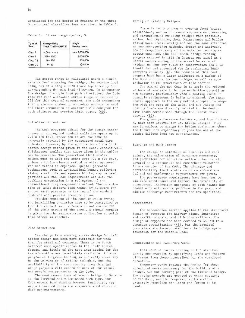
considered tor the design ot bridges on the three Ontario road classifications are given in Table 4.

Table 4. Stress range cycles, N.

Type of Average Daily Single Road Truck Traffic (ADTT) Service Loads

Class A 1000 or more over 2,000,000

Class 8 250 - 1000 2,000,000

Class C-1 50 - 250 500,000

Class C-2 0- 50 100,000

The stress range is calculated using a single service load crossing the bridge, the service load being 80% of a single OHBD Truck amplified by the corresponding dynamic load allowance. To discourage the design of single load path structures, the Code requires that allowable stress range be reduced by 25% for this type of structure. The Code emphasizes that a minimum number of secondary members be used and their components be appropriately designed for both ultimate and service limit states ~).

Soil-Steel Structures

The Code provides tables for the design thick­nesses of corrugated conduit walls for spans up to 7.9 m (26 ft.). These tables are the same as presently provided by the corrugated metal pipe industry. However, by the application of the limit states design method given in the Code, conduit wall thicknesses smaller than those given in the tables may be possible. The prescribed limit states method must be used for spans over 7.9 m (26 ft.), unless a finite element method or other approved refined method is employed. Special patented

' techniques, such as longitudinal beams, relieving slabs, steel ribs and squeeze blocks, may be used provided all the Code requirements are met. The buckling computation is a ref i~ment of the conventional ring compression method. The calcula­tion of loads differs from AASHTO by allowing for active earth pressure on the top of the conduit combined with passive pressure below.

The deformations of the conduit walls during the backfilling operation have to be controlled so that the conduit wall stresses do not exceed 90% of the yield stress of the steel. A simple formula is given for the maximum crown deflection at which this stress is reached.

,-y __ ..J {"' ..... _____ .._ _____ _

WUUU UL.l.UCLUJ...et::i

The change from working stress design to limit states design has been more difficult for wood than for steel and concrete. There is no North American wood specification in the limit states format, and little of the test data needed for the transformation was immediately available. A large program of in-grade testing is currently under way at the University of British Columbia, and the availability of the test results from this and other projects will determine many of the values and provisions appearing in the Code.

The most common form of wooden bridge in Ontario is the longitudinally laminated deck type. The Code covers load sharing between laminations for asphalt covered decks and composite wood-concrete deck superstructures.

Rating of Existing Bridges

There is today a growing concern about bridge maintenance, and an increased emphasis on preserving and strengthening existing bridges when possible, rather than replacing them. Maintenance and bridge rating have traditionally not had the same attention as new construction methods, design and analysis, and in comparison many of the existing techniques appear outdated. The full-scale hridge testine program started in 1969 in Ontario was aimed at a better understanding of the actual behavior of bridges so that any built-in conservatism could be identified and accounted for in evaluating load­carrying capacity (6). The results of this test program have had a l arge influence on a number of the Code sections for new bridges as well as con­tributing to the provisions of this section.

The aim of the new Code is to apply the refined methods of analysis to bridge evaluation as well as new designs, particularly when a posting limit or possible replacement is being considered. The limit states approach is the only method accepted in keep­ing with the rest of the Code, and the rating and posting loads are directly related to the design live loads established through the latest truck surveys (16).

The given performance factors ~. and load factors K, have been derived for new bridge designs. They may be subject to change for bridge evaluation where the future life expectancy or possible use of the bridge differs from new construction.

Bearings and Deck Joints

The design or selection of bearings and deck joints, the calculation of structure movements, and provisions for structure articulation are all covered in a systematic and comprehensive manner in one section of the Code. The ultimate and serviceability limit states to be considered are defined and performance requirements are given.

The performance requirements have been set to minimize maintenance and improve the durability of structures. Inadequate anchorage of deck joints has caused many maintenance problems in the past, and minimum anchorage requirements are now specified.

Accessories

The accessories section applies to the structural design of supports for highway signs, luminaires and traffic signals, and of bridge railings. The design of supports has been covered by AASHTO in a separate specification(~, but the required provisions are incorporaced inco che bridge spec­ification for the Ontario Code.

Construction and Temporary Works

This section covers loading of the structure during construction by specifying loads and factors different from those prescribed for the completed structure.

Temporary works include the design for those structural works necessary for the building of a bridge, but not forming part of the finished bridge. The design methods are covered by other sections of the Code, and the temporary works section primarily specifies the loads and forces to be used.

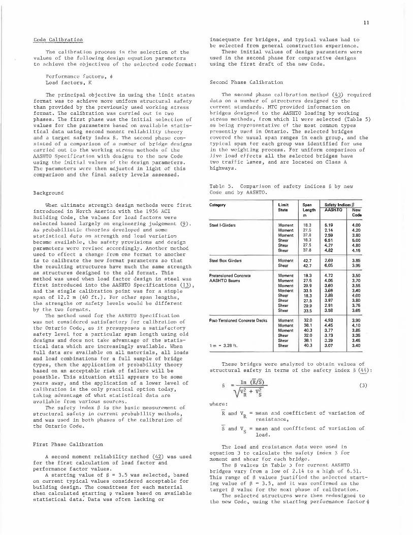
Code Calibration

The calibration process is the selection of the values of the following design equation parameters to achieve the objectives of the selected code format:

Performance factors, 4 Load factors, K

The principal objective in using the limit states format was to achieve more uniform struc tural safety than provided by the previously used working stress format. The calibration was carried out in two phases. The first phase was the initial selection of values for the parameters based on available statis­tical data using second moment reliability theory and a target safety index 8. The second phase con­sisted of a comparison of a number of bridge designs carried out to the working stress methods of the AASHTO Specification with designs to the new Code using the initial values of the design parameters. The parameters were then adjusted in light of this comparison and the final safety levels assessed.

Background

When ultimate strength design methods were first introduced in North America with the 1956 ACI Building Code, the values for load factors were selected based largely on engineering judgement (_2). As probabilistic theories developed and some statistical data on strength and load variation became available, the safety provisions and design parameters were revised accordingly. Another method used to effect a change from one format to another is to calibrate the new format parameters so that the resulting structures have much the same strength as structures designed to the old format. This method was used when load factor design in steel was first introduced into the AASHTO Specifications (13), and the single calibration point was for a simple~ span of 12.2 m (40 ft,). For other span lengths, the strengths or safety levels would be different by the two formats.

The method used for the AASHTO Specification was not considered satisfactory for calibration of the Ontario Code, as it presupposes a satisfactory safety level for a particular span length using old designs and does not take advantage of the statis­tical data which are increasingly available. When full data are available on all materials, all loads and load combinations for a full sample of bridge types, then the application of probability theory based on an acceptable risk of failure will be possible. This situation still appears to be some years away, and the application of a lower level of calibration is the only practical option today, taking advantage of what statistical data are available from various sources.

The safety index 8 is the basic measurement of structural safety in current probability methods, and was used in both phases of the calibration of the Ontario Code.

First Phase Calibration

A second moment reliability method (42) was used for the first calculation of load f actor--and performance factor values.

A starting value of 8 = 3.5 was selected, based on current typical values considered acceptable for building design. The committees for each material then calculated starting 4 values based on available statistical data: Data was often lacking or

inadequate for bridges, and typical values had to be selected from general construction experience.

These initial values of design parameters were used in the second phase for comparative designs using the first draft of the new Code.

Second Phase Calibration

11

The second phase calibration method (43) required data on a number of structures designed t~the current standards. MTG provided information on bridges designed to the AASHTO loading by working stress methods, from which 11 were selected (Table 5) as being representative of the most common typ es presently used in Ontario. The selected bridges covered the usual span ranges in each group, and the typical span for each group was identified for use in the weighting process. For uniform comparison of live load effects all the selected bridges have two traffic lanes, and are located on Class A highways.

Table 5. Comparison of safety indices 8 by new Code and by AASHTO.

Category Limit Sp en Safety Indices ll State Length AASHTO New

m Code

Steel I-Girders Moment 18.3 5.19 4.00 Moment 27.5 2.14 4.20 Moment 37.8 2.59 3.80 Shear 18.3 6.51 5.00 Shear 27.5 4.27 4.80 Shear 37.8 4.82 4.15

Steel Box Girders Moment 42 .7 2.69 3.85 Shear 42.7 6.05 3.95

Pretensioned Concrete Moment 18.3 4.72 3.50 AASHTO Beams Moment 27.5 4.05 3.70

Moment 29.9 3.60 3.55 Moment 33.5 3.66 3.40 Shear 18.3 2.88 4.00 Shear 27 .5 3.97 3.80 Shear 29.9 2.91 3.75 Shear 33.5 3.58 3.65

Post-Tensioned Concrete Decks Moment 32.0 4.93 3.90 Moment 38.1 4.45 4.10 Moment 40.3 3.77 3.85 Shear 32.0 3.73 3.35 Shear 38.1 3.29 3.45

1 m = 3.28 ft . Shear 40.3 3.07 3.40

These bridges were analyzed to obtain values of structural safety in terms of the safety index 8 (44):

where:

lo (i/s)

yv~ + v~ (3)

mean and coefficient of variation of resistance,

mean and coefficient of variation of load.

The load and resistance data were used in equation 3 to calculate the safety index 8 for moment and shear for each bridge.

The 8 values in Table 5 for current AASHTO bridges vary from a low of 2.14 to a high of 6.51. This range of 8 values justified the selected start­ing value of 8 = 3.5, and it was confirmed as the target 8 value for the next phase of calibration.

The selected structures were then redesigned to the new Code, using the starting performance factor 4

1 2

values given by the sub-committees, and the starting load factor K values from the firs t phase calibration.

The objective of the subsequent calibration process (.'.!2_) was to reduce the .scatter of B values by adjustment of the starting values of the design equation parameters. With the calibrated values of these parameters, the B values were recalculated to check the variation from the target value of 3 .5. The results ar e shown in Table 5, and the B value s~AttAr has been reduced to between 3 .35 and ~.2 (45), except for steel girders in shear .

These calibrated values of the design parameters were us ed i n the draft of the Code distributed for public comment, and are shown in Tables 6 and 7. The values may be changed as further calibration work is performed , before the Code is published.

Table 6. Calibrated values of load fac tor s K.

Load Factor Description

Live Load KL .

Dynamic Load Allowance K1.

Dead Load K01

for fectory produced structural componC! nts.

Dead Load K0 2 far C<>st-in·IT•ld structural components and all non-s tructural components.

Dead Load K03

for ssphalt wearing surfeco .

Load Factor Values

1.35

1.35

1.15

1.25

1.7

Table 7. Calibrated values of performance factors ~.

Category Limit </> Value State

Steel Girders Moment 0.90 Shear 0.90

Pretensioned Concrete Beams Moment 0.85 Shear 0.65

Post-Tensioned Concrete Decks Moment 0.85 Shear 0.65

Closing Remarks

The Ontario Highway Bridge Design Code will be published in late 1978, and work wil l then begin on a revised edition to be issued one year later.

The primary objective of the change to Limit States Format - the provision of more uniform safety levels - appears to have been achieved. Whether improved economy has also been attained can only be ass essed when an adequate sample of bridges has been designed to the new Code . How­ever, it is expected that the increased design live load can be accommodated and s till produce a 10% saving in structural materials.

References

I. Standard Specifications for Highway Bridges. AASHTO 1977. 2. CSA Standard S6-1974. Design of Highway Bridges. 3. P.F. Csagoly and R.A. Dorton. Proposed Ontario Bridge Design Load.

MTC, RR186, 1973. 4. R.A. Dorton,M. HolowkaandJ.P.C. King. The Conestoga River Bridge -

Design and Testing. CJCE, Vol. 4, No. !,March 1977. 5. J.P.C. King, M. Holowka, R.A. Dorton and A.C. Agarwal. Test Results

from theConestogo River Bridge.Bridge Engineering Conf. , TRB, 1978. 6. B. Bakht and P.F. Csagoly. Testing of Perley Bridge. Research and

Development Division, MTC, 1977, RR207.

7. ACI Comm. 318. Building Code Requirements for Reinforced Concrete. ACl-318-63, 1963.

8. National Building Code. NRC, 1975. 9. J.G. MacGregor. Safety and Limit States Design for Reinforced Concrete.

CJCE, Vol. 3, No. 4, 1976. 10. D.J.L. Kennedy . Limit States Design - An Innovation in Design

S1andards for S1eel S1ructures. CJCE, Vol. 1, No. I, 1974. 11. D.E. Allen. Limit States Design - A Probabilistic Study. CJCE, Vol. 2 ,

No. I, 1975. 12. ACI Comm. 443 . Analysis and Design of Reinforced Concrete Bridge

Structures. 1977. 13. G .S. Vincent. Tenta1ive Criteria for Load Factor Design of Steel Highway

Bridges. American Iron and Steel Inst. N.Y., February 1968. 14. F.W. Jung and A.A. Witecki. Determining the Maximum Permissible

Weights of Vehicles on Bridges. MTC, RR! 75 , 1971. 15 . D. Harman and A.G. Davenport. The Formulation of Vehicular Loading

for the Design of Highway Bridges in Ontario. U. of Western Ontario, December, 1976.

16. A.C. Agarwal and P.F. Csagoly. Evaluation and Posting of Bridges in Ontario. Bridge Engineering Conf. TRB, 1978.

17. R.N. Wright and W.H. Walker. Vibration and Deflection of Steel Bridges. AISC Engineering Journal. January 1972.

18. D.T. Wright and R. Green. Human Sensitivity to Vibration. Ontario Joint Highway Research Program Report. February 1958.

19. D.T. Wright and R. Green. Highway Bridge Yibrations. Ontario Joint Highway Research Program Report. May 1964.

20. R . Green. The Motion of Highway Bridges under Moving Loads . MSc Thesis, Queen's University, 1958.

21. P.F. Csagoly, T.I. Campbell and A.C. Agarwal. Bridge Vibration Study. MTC, RR 181, 1972.

22. H. Reigher and F.J. Meister. The Effect of Vibration and People. Hq. Air Material Command, Wright Field, Ohio, 1946, F-TS-616-RE.

23. B. Bakht and R.C. Bullen. Analysis of Orthotropic Right Bridge Decks. Dept. or the Environment , London, Eng., 1974. HECB/B/15 (ORTHOP).

24. B. Onkht, P.F. Cs;igoly im<I C. Jaeger. Effect ofComp11terson Economy of Bridge Design. Proc. of the CSCE Specialty Conf. on Computers in Structural Engineering Practice. Montreal, October 1977.

25. D.W. Smith. Bridge Failures. Proc. of the Institution of Civil Engineers . U.K., August 1976.

26. J .F. Brotchie and M.H. Holley. Membrane Action in Slabs. AC!, Detroit. SP-30, 1971.

27. P.Y. Tong and B. deV. Batchelor. Compressive Membrane Enhancement in Two-Way Bridge Slabs. AC!, De1roit. SP-30, 1971.

28. B. deV. Batchelor, B.E. Hewitt, P.F. Csagoly and M. Holowka. An Investigation of the Ultimate Strength of Occk Slabs of Composite Steel/Concrete Bridges. Bridge Engineering Conf. TRB, 1978.

29. P .F. Csagoly, M. Holowka and R.A. Dorton . The True Behavior of Thin Concrete Bridge Decks. Bridge Engineering Conf. TRB, 1978.

30. ACI Comm. 318. Building Code Requirements for Reinforced Concrete. ACl-318-71, 1971.

31. ACI-ASCE Comm. 426. Suggested Revisions to Shear Provisions of Building Codes. AC! Journal, Vol. 74, No. 9. September 1977.

32. ACI-ASCE Comm. 426. The Shear Strength of Reinforced Concrete Mem­bers. Journal of the Structural Div., ASCE. Vol. 99, No. ST 6, June 1973.

33. Code for the Design of Concrete Structures for Buildings. CSA Standard . A23.3-1973. CSA, Ontario , 1973.

34. P. Lampert and M.P. Collins . Torsion, Bending and Confusion - An Attempt to Eslnb!ish !he Facts . ACI Journal, Vol. 69, No. 8. Aug. 1972.

35. P .F. Cs<1go ly and M. Holowka. Cracking of Voided Post-Tensioned Concrete Decks. MTC, RR 193, 1974.

36. L. Chilnuyanondh. Shear F llute llf Concrete I-Beams with Pres tressing Ducts in the Web. PhD Thesis, Queen's University, 1976.

37. S.T. Rolfe. Fracture MechHnic.s an rl the AASHTO M•teria! Toughness Requirements for Bridge Steels. Proc. CSE Conf. 1976. Canadian Steel Industries Construction Council, Toronto.

38 . Steel Structures for Buildings, Limit States Design. CSA Standard S!6.l-1974. CSA, Ontario, 1974.

39. Limit States Design Steel Manual, Canadian Institute for Steel Construct­ion, Toronto, 1977.

40. J.W. Fisher, A.W. Pense and R. Roberts. Evaluation of Fracture of Lafayette Street Bridge. Journal of the Structural Div., ASCE, Vol. 103, No. ST 7, July 1977.

41. Standard Specifications for Structural Supports for Highway Signs, Luminaires and Traffic Signals. AASHTO, I 975.

42. M.K. Ravindra, N.C . Lind and W.C. Siu. Illustrations of Reliability Based Design . Journal of the Structural Div. ASCE, Vol. JOO , No. ST 9, September 1974.

43. W.C. Siu, S.R. Parimi and N.C. Lind. Practical Approach to Code Calibra­tion. Journal of the Structurnl Div., ASCE, Vol. I 01, No. ST 7, July 1975.

44. E. Roscnblueth and L. Estcva. Reliabilll::' Basis for Some Mexican Codes. ACI , Detroit. Publication SP-3 I , 1972.

45. A.S. Nowak and N.C. Lind . Calibration of the OHB Design Code. On1ario Highway Bridge Design Code Report. University of Waterloo. 1977.