1

The Use of Smart Meter Data to ForecastElectricity Demand

Armin Haghi, Oliver TooleCS229 Course project, Fall 2013

I. MOTIVATION

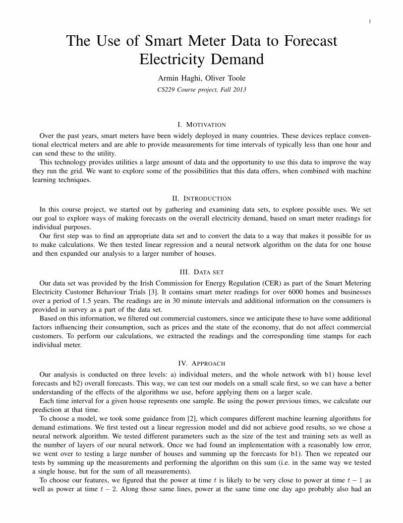
Over the past years, smart meters have been widely deployed in many countries. These devices replace conven-tional electrical meters and are able to provide measurements for time intervals of typically less than one hour andcan send these to the utility.

This technology provides utilities a large amount of data and the opportunity to use this data to improve the waythey run the grid. We want to explore some of the possibilities that this data offers, when combined with machinelearning techniques.

II. INTRODUCTION

In this course project, we started out by gathering and examining data sets, to explore possible uses. We setour goal to explore ways of making forecasts on the overall electricity demand, based on smart meter readings forindividual purposes.

Our first step was to find an appropriate data set and to convert the data to a way that makes it possible for usto make calculations. We then tested linear regression and a neural network algorithm on the data for one houseand then expanded our analysis to a larger number of houses.

III. DATA SET

Our data set was provided by the Irish Commission for Energy Regulation (CER) as part of the Smart MeteringElectricity Customer Behaviour Trials [3]. It contains smart meter readings for over 6000 homes and businessesover a period of 1.5 years. The readings are in 30 minute intervals and additional information on the consumers isprovided in survey as a part of the data set.

Based on this information, we filtered out commercial customers, since we anticipate these to have some additionalfactors influencing their consumption, such as prices and the state of the economy, that do not affect commercialcustomers. To perform our calculations, we extracted the readings and the corresponding time stamps for eachindividual meter.

IV. APPROACH

Our analysis is conducted on three levels: a) individual meters, and the whole network with b1) house levelforecasts and b2) overall forecasts. This way, we can test our models on a small scale first, so we can have a betterunderstanding of the effects of the algorithms we use, before applying them on a larger scale.

Each time interval for a given house represents one sample. Be using the power previous times, we calculate ourprediction at that time.

To choose a model, we took some guidance from [2], which compares different machine learning algorithms fordemand estimations. We first tested out a linear regression model and did not achieve good results, so we chose aneural network algorithm. We tested different parameters such as the size of the test and training sets as well asthe number of layers of our neural network. Once we had found an implementation with a reasonably low error,we went over to testing a large number of houses and summing up the forecasts for b1). Then we repeated ourtests by summing up the measurements and performing the algorithm on this sum (i.e. in the same way we testeda single house, but for the sum of all measurements).

To choose our features, we figured that the power at time t is likely to be very close to power at time t− 1 aswell as power at time t − 2. Along those same lines, power at the same time one day ago probably also had an

2

Variable Description

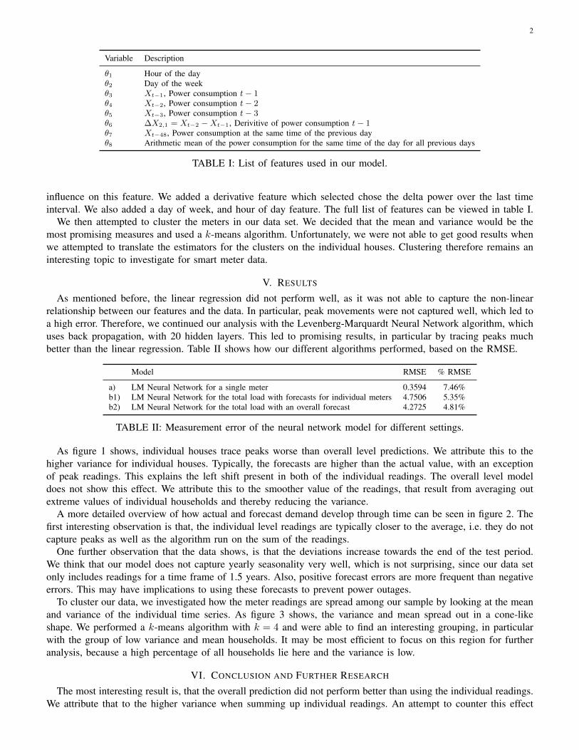
θ1 Hour of the dayθ2 Day of the weekθ3 Xt−1, Power consumption t− 1θ4 Xt−2, Power consumption t− 2θ5 Xt−3, Power consumption t− 3θ6 ∆X2,1 = Xt−2 −Xt−1, Derivitive of power consumption t− 1θ7 Xt−48, Power consumption at the same time of the previous dayθ8 Arithmetic mean of the power consumption for the same time of the day for all previous days

TABLE I: List of features used in our model.

influence on this feature. We added a derivative feature which selected chose the delta power over the last timeinterval. We also added a day of week, and hour of day feature. The full list of features can be viewed in table I.

We then attempted to cluster the meters in our data set. We decided that the mean and variance would be themost promising measures and used a k-means algorithm. Unfortunately, we were not able to get good results whenwe attempted to translate the estimators for the clusters on the individual houses. Clustering therefore remains aninteresting topic to investigate for smart meter data.

V. RESULTS

As mentioned before, the linear regression did not perform well, as it was not able to capture the non-linearrelationship between our features and the data. In particular, peak movements were not captured well, which led toa high error. Therefore, we continued our analysis with the Levenberg-Marquardt Neural Network algorithm, whichuses back propagation, with 20 hidden layers. This led to promising results, in particular by tracing peaks muchbetter than the linear regression. Table II shows how our different algorithms performed, based on the RMSE.

Model RMSE % RMSE

a) LM Neural Network for a single meter 0.3594 7.46%b1) LM Neural Network for the total load with forecasts for individual meters 4.7506 5.35%b2) LM Neural Network for the total load with an overall forecast 4.2725 4.81%

TABLE II: Measurement error of the neural network model for different settings.

As figure 1 shows, individual houses trace peaks worse than overall level predictions. We attribute this to thehigher variance for individual houses. Typically, the forecasts are higher than the actual value, with an exceptionof peak readings. This explains the left shift present in both of the individual readings. The overall level modeldoes not show this effect. We attribute this to the smoother value of the readings, that result from averaging outextreme values of individual households and thereby reducing the variance.

A more detailed overview of how actual and forecast demand develop through time can be seen in figure 2. Thefirst interesting observation is that, the individual level readings are typically closer to the average, i.e. they do notcapture peaks as well as the algorithm run on the sum of the readings.

One further observation that the data shows, is that the deviations increase towards the end of the test period.We think that our model does not capture yearly seasonality very well, which is not surprising, since our data setonly includes readings for a time frame of 1.5 years. Also, positive forecast errors are more frequent than negativeerrors. This may have implications to using these forecasts to prevent power outages.

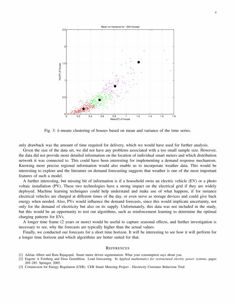
To cluster our data, we investigated how the meter readings are spread among our sample by looking at the meanand variance of the individual time series. As figure 3 shows, the variance and mean spread out in a cone-likeshape. We performed a k-means algorithm with k = 4 and were able to find an interesting grouping, in particularwith the group of low variance and mean households. It may be most efficient to focus on this region for furtheranalysis, because a high percentage of all households lie here and the variance is low.

VI. CONCLUSION AND FURTHER RESEARCH

The most interesting result is, that the overall prediction did not perform better than using the individual readings.We attribute that to the higher variance when summing up individual readings. An attempt to counter this effect

3

0 10 20 30 40 50 60 70 80 90 1000

10

20

30

40

50

60

70

80

90

100

Forecast (kW)

Actu

al R

ea

din

gs (

kW

)

0 1 2 3 4 5 60

1

2

3

4

5

6

Forecast (kW)

Actu

al R

ea

din

gs (

kW

)

Single Level PredictionsHouse Level Predictions

Overall Level Predictions

Fig. 1: Comparision of predictions with Actual vs Forecast data.

0 1000 2000 3000 4000 5000 6000 7000 80000

20

40

60

80

100

Time (half hours)

Po

we

r (k

W)

Overall vs House level predictions

Actual

House level predictions

Overall prediction

0 1000 2000 3000 4000 5000 6000 7000 8000−20

−10

0

10

20

30

time (half hours)

Err

or

Forecast errors

House error

Overall error

Fig. 2: Overall vs House level predictions.

and find a better result on a middle ground would be to perform clustering on the individual households to findthe predictors and to perform the forecasts with these, rather than on a truly individual level forecast. Some work,such as [1], has already been done on the classification of households, which could potentially be useful.

The focus of this study was to test what techniques are useful when working with time series data from smartmeters. We did not worry about implementing the algorithms, but a real life solution may require putting the systemin an online learning algorithm. It is also necessary to find a way to deal with the addition or removal of meters.For our study, the data included readings for all households over the whole period, this is not the case in reality.

Due to privacy concerns, it is still very difficult to get good data sets and even more difficult to find a testingenvironment (e.g. to test controlling power generation). Our data set was very useful in many ways, since itprovides realistic and broad data, compared to some data sets that have very short intervals and few houses. The

4

0 0.2 0.4 0.6 0.8 1 1.2 1.4 1.6 1.80

0.5

1

1.5

2

2.5

Mean(P) of house

Va

r(P

) o

f h

ou

se

Mean vs Variance for ~500 houses

Fig. 3: k-means clustering of houses based on mean and variance of the time series.

only drawback was the amount of time required for delivery, which we would have used for further analysis.Given the size of the data set, we did not have any problems associated with a too small sample size. However,

the data did not provide more detailed information on the location of individual smart meters and which distributionnetwork it was connected to. This could have been interesting for implementing a demand response mechanism.Knowing more precise regional information would also enable us to incorporate weather data. This would beinteresting to explore and the literature on demand forecasting suggests that weather is one of the most importantfeatures of such a model.

A further interesting, but missing bit of information is if a household owns an electric vehicle (EV) or a photovoltaic installation (PV). These two technologies have a strong impact on the electrical grid if they are widelydeployed. Machine learning techniques could help understand and make use of what happens, if for instanceelectrical vehicles are charged at different times of the day, or even serve as storage devices and could give backenergy when needed. Also, PVs would influence the demand forecasts, since this would implicate uncertainty, notonly for the demand of electricity but also on its supply. Unfortunately, this data was not included in the study,but this would be an opportunity to test out algorithms, such as reinforcement learning to determine the optimalcharging patterns for EVs.

A longer time frame (2 years or more) would be useful to capture seasonal effects, and further investigation isnecessary to see, why the forecasts are typically higher than the actual values.

Finally, we conducted our forecasts for a short time horizon. It will be interesting to see how it will perform fora longer time horizon and which algorithms are better suited for that.

REFERENCES

[1] Adrian Albert and Ram Rajagopal. Smart meter driven segmentation: What your consumption says about you.[2] Eugene A Feinberg and Dora Genethliou. Load forecasting. In Applied mathematics for restructured electric power systems, pages

269–285. Springer, 2005.[3] Commission for Energy Regulation (CER). CER Smart Metering Project - Electricity Customer Behaviour Trial.