1. Shocks - MIT OpenCourseWare · the quarter). Leaves 10 parameters (6 parameters, and 4 standard deviations). 10 moments in Ω. Non linear system. Alternative, and more intuitive:

1. Shocks

Nr. 1

Cite as: Olivier Blanchard, course materials for 14.462 Advanced Macroeconomics II, Spring 2007. MIT OpenCourseWare (http://ocw.mit.edu/), Massachusetts Institute of Technology. Downloaded on [DD Month YYYY].

1.2. Structural VARs

How to identify A0? A review:

Choleski (Cholesky?) decompositions. •

Short-run restrictions. •

Inequality restrictions. •

Long-run restrictions. •

Then, examples, applications, and conclusions:

BQ Gali: Mix of short-run and long-run restrictions •

Uhlig: inequality constraints. •

Nr. 2


True model:

X = (A0 + A1 L + A2 L2 + ...) e = A(L)e; E(ee�) = I

Estimated model:

X = (u + C1 L + C2 L2 + ...) u = C(L)u; E(uu�) = Ω

Implication: u = A0e A0A

�0 = Ω ⇒

Identification 1. Choleski orderings and decomposition

There exists a unique lower triangular matrix S such that SS� = Ω. Can useit. One for each ordering of the variables in u.Does it make sense? Sometimes:

Nr. 3


A supply-demand example. P , Q; p, q VAR residuals, es, ed true shocks tosupply and demand.If price set in advance by price-setters:

p = a11 es ; q = a21 es + a22 ed

This corresponds to a Choleski ordering, with p first (a12 = 0) �

a11 0 �

A0 = a21 a22

Simplest way to estimate the VAR:

p on lagged ps and lagged qs. gives es•

q on current p, lagged ps, and lagged qs. gives ed•

Nr. 4


If quantity supplied is set in advance

q = a11 es ; p = a21 es + a22 ed

This corresponds to a Choleski ordering, with q first (a12 = 0) Simplest way to estimate the VAR:

q on lagged ps and lagged qs. gives es•

p on current q, lagged ps, and lagged qs. gives ed.•

But, in general, useless without a structural interpretation.

Nr. 5


Identification 2. Short-run restrictions

Zero restrictions or parameters set from other information, for A0. Example from Blanchard-Watson, 1987:

Four variables Y, P, G,M . VAR residuals y, p, g, m. Four underlying shocks es, ed, eg, em . Four postulated relations: AS, AD, fiscal and monetary rules:

AS y = b1 p + σs e s

AD y = b2 m − b3 p + b4 g + σd e d

g = c1 y + c2 p + σg eg

m = c3 y + c4 p + σm e m

Get c1, c2 from tax and spending rules (no discretionary fiscal policy within the quarter). Leaves 10 parameters (6 parameters, and 4 standard deviations). 10 moments in Ω.

Non linear system. Alternative, and more intuitive: IV approach: eg as an IV for p in AS, es and eg as IV in money rule, em, eg, es as IV in AD.

Nr. 6


Identification 3. Inequality restrictions

Back to supply-demand system. May be reasonable to assume a range ofprice-elasticity for supply.For a given price-elasticity, and uncorrelated supply and demand shocks, canestimate demand. And draw impulse responses.

Uhlig’s 2004 application to monetary policy shocks.

Useful detour: Note that any A0 must be an orthogonal transformation of theCholeski matrix S. Assume A0 = SQ for arbitrary matrix Q. Then:

A0A�0 = SQQ�S� = Ω QQ� = I⇔

An orthogonal matrix has orthogonal rows (and columns) and row and column lengths equal to one.

Nr. 7 Cite as: Olivier Blanchard, course materials for 14.462 Advanced Macroeconomics II, Spring 2007. MIT OpenCourseWare (http://ocw.mit.edu/), Massachusetts Institute of Technology. Downloaded on [DD Month YYYY].

In 2x2 case, an orthogonal matrix can be parameterized by one parameter:

� cos(θ) − sin(θ)

� � cos(θ) sin(θ)

�Q = or sin(θ) cos(θ) sin(θ) − cos(θ)

Uhlig: All values of θ such that the impulse response function associated with a given A0 = S Q(θ) and A(L) = C(L) A0 satisfy some condition.

Variables: Real GDP, GDP deflator, commodity price index, total reserves,nonborrowed reserves, federal funds rate, monthly 1965-1996. (How is real GDP constructed?)

Condition: Responses to a (negative) monetary policy shock: non-borrowed reserves and price level non positive; federal funds rate, non negative, up to K = 5.


Bayesian interpretation. Uniform prior on θ that satisfy the constraint.•

Uhlig identifies only one shock. But method can be used for a full• decomposition.

No constraint on response of GDP. Focus of paper.•

Results. Not very good news for monetary policy: Figure 7, and figure • 12 (real output response constrained to zero at K = 0).


Image removed due to copyright restrictions.

Figure 7: Impulse responses of real GDP to a contractionary monetary policy shock one standard deviation in size, using the pure-sign-restriction approach. ��

Uhlig, H. "What are the effects of monetary policy on output? Results from an agnostic identification procedure."mimeo Humboldt University, May 2004. p. 42. (http://www2.wiwi.hu-berlin.de/institute/wpol/papers/uhlig_effects-monetarypolicy-output.pdf)


Image removed due to copyright restrictions.��

Figure 12: Impulse responses to a contractionary monetary policy shock one standard deviation in size, using the pure-sign-restriction approach with K=5, additionally imposing a zero response on impact for real GDP. ��

Uhlig, H. "What are the effects of monetary policy on output? Results from an agnostic identification procedure." mimeo Humboldt University, May 2004. p. 47. (http://www2.wiwi.hu-berlin.de/institute/wpol/papers/uhlig_effects-monetarypolicy-output.pdf)


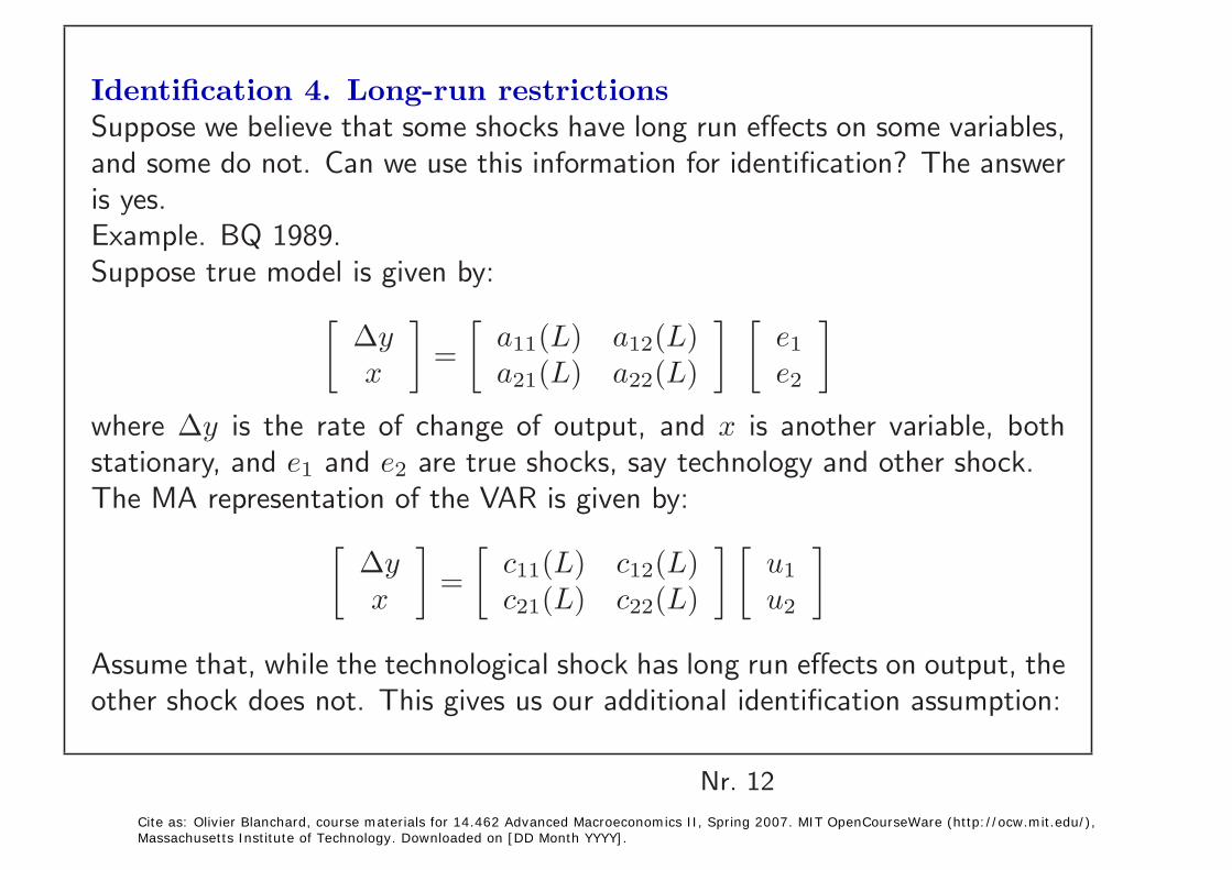
Identification 4. Long-run restrictions Suppose we believe that some shocks have long run effects on some variables,and some do not. Can we use this information for identification? The answeris yes.Example. BQ 1989.Suppose true model is given by:

� Δy

�

=

� a11(L) a12(L)

� � e1

�

x a21(L) a22(L) e2

where Δy is the rate of change of output, and x is another variable, both stationary, and e1 and e2 are true shocks, say technology and other shock. The MA representation of the VAR is given by:

� Δy

�

=

� c11(L) c12(L)

� � u1

�

x c21(L) c22(L) u2

Assume that, while the technological shock has long run effects on output, theother shock does not. This gives us our additional identification assumption:


The restriction on the true model is:

[A(1)]12 = 0

As A(L) = C(L) A0, Ω = S S�, and A0 = SQ, these imply:

[C(1)A0]12 = [C(1)SQ]12 = 0

From estimation, we have estimates of C(1) and S, so all we have to do is to solve for Q, equivalently for the free parameter θ.

Then, same steps as before.

How to choose the second variable (or the set of other variables than technology)? Has to be affected by both shocks, be stationary. BQ: U rate. But, if only two shocks, any other variable should give same results...

Nr. 13


Potential problems with LR identification restrictions? (maintained assumption: Two shocks, one with permanent effects, the other not.)

Imposing a zero frequency restriction. Sample size is finite. •

• Potential truncation bias from VAR estimation (Chari-Kehoe-McGrattan)

Small sample bias. •

Non linear mapping from C(L) and Ω to A0. (Should show up in • bootrapped sd bands)

No general results. Study of RBC and NK models by Erceg-Gerrieri-Gust 2005.


A first picture. BQ 1989 and Gali 1992

• BQ 1989: First difference of log GDP, and unemployment rate. US, quarterly, 1950:1 to 1987:4.

• Practical issues: With/without time trend for unemployment, dummy break for growth rate in 1974:1

Impulse responses. Figures 3 to 6. (bootstrapped one-sd bands)•

“Other” (demand?) shocks: Hump shaped positive response of output, negative response of unemployment.

Technology shocks: Slow increase in output, initial increase in unemployment. Interpretation?

• Variance decompositions. Tables 2a to 2d. At 4 quarters, demand accounts for 87.9% (trend, dummy) to 38.9% (no trend, no dummy) of movements in GDP. (90% to 80% of movements in unemployment)

• Output due to tech shocks ≡ natural output? No.


Image removed due to copyright restrictions.��

Figures 3 to 6. p. 663 in Blanchard, Olivier, and Danny Quah. "The Dynamic Effects of Aggregate Demand and Supply Disturbances." American Economic Review 79, no. 4 (Sep. 1989): 655-673.


Image removed due to copyright restrictions.�

Tables 2 to 2A. p. 666.

Blanchard, Olivier, and Danny Quah. "The Dynamic Effects of Aggregate Demand and Supply Disturbances." American Economic Review 79, no. 4 (Sep. 1989): 655-673.



Tables 2B to 2C. p. 667.

Blanchard, Olivier, and Danny Quah. "The Dynamic Effects of Aggregate Demand and Supply Disturbances." American Economic Review 79, no. 4 (Sep. 1989): 655-673.

Nr. 18


Gali 1999, with extensions in Gali and Rabanal 2004. (Leave the formal model aside for the time being. Back to it later)

Benchmark: •

Two variables. Labor productivity, and total hours (logs, so implicitlylog GDP as well).

Two shocks. One (technology) with permanent effects on labor productivity. The other (non-technology) without permanent effects of laborproductivity. Both shocks may/may not have long run effects on hours.

Relation and differences with BQ: Labor productivity rather than out• put. Excludes (permanent) labor supply shocks. Labor productivity and technological shocks: Stationarity of the capital-output ratio?

Benchmark: US, quarterly, 1948:1 to 1994:4. Two specifications: Unit • root and first differences in hours, or deviations of hours from deterministic trend.

(Interpretation of non-technology shock in first case?)


Results: Figures 2 and 3 (2-sd bands)

Favorable technological shocks lead to steady increase in output, and • an initial decrease in hours.

Favorable non-technology shocks lead to an initial increase in produc• tivity, largely gone after a year, and a steady increase in hours, largely permanent (in the first difference version).

Non-technology shock component of GDP tracks the behavior of GDP • (HP filtered) very well.

Nr. 20



Figure 2: Estimated Impulse Responses from a Bivariate Model. p. 261.Gali, J. "Technology, employment and the business cycle: Do technology shocks explain aggregate fluctuations?" American Economic Review 89, no. 1 (1999): 249-271.



Figure 3: Estimated Impulse Responses from a Bivariate Model. p. 262. Gali, J. "Technology, employment and the business cycle: Do technology shocks explain aggregate fluctuations?"

American Economic Review 89, no. 1 (1999): 249-271.



Figure 1: Productivity vs. Hours. p. 260. Gali, J. "Technology, employment and the business cycle: Do technology shocks explain aggregate fluctuations?" American Economic Review 89, no. 1 (1999): 249-271.



Figure 6: Estimated Technology and Nontechnology Components of U. S. GDP and Hours. p. 268.Gali, J. "Technology, employment and the business cycle: Do technology shocks explain aggregate fluctuations?" American Economic Review 89, no. 1 (1999): 249-271.��


Extension 1. More variables. •

Why? If more than one non-technology shock. Can still identify the technology shock, if the only one to have permanent effects on productivity. No need to identify each of the others.

Add real balances, real interest rates, and inflation. Similar results.

Extension 2. Other countries. •

Very useful, for two reasons. Darwinian effects at work on US data. Possibly different shocks (think Chile, or Norway). Here, just major OECD countries. (Δy/n, Δn for all countries except France (detrended n)

Good news: Consistency: In all countries, technology shocks lead to an increase in output, an initial decrease in hours.

Potentially less good news: Tech shocks: No build-up of output over time. LR effects of non-tech shocks on employment.



Figure 5: Estimated Impulse Responses of Employment and Productivity for Other Industrialized Economies. p. 266. Gali, J. "Technology, employment and the business cycle: Do technology shocks explain aggregate fluctuations?" American Economic Review 89, no. 1 (1999): 249-271.



Figure 5 continued. Estimated Impulse Responses of Employment and Productivity for Other Industrialized Economies. p. 267.Gali, J. "Technology, employment and the business cycle: Do technology shocks explain aggregate fluctuations?" American Economic Review 89, no. 1 (1999): 249-271.��

Nr. 27


Taking stock and what comes next.

Structural VARs best used when class of models in mind. Does the class • fit, and what does this suggest about the parameters? (Nice example away from macro: Job market paper by Kline on effects of oil prices on labor market in Texas)

If too broad (few constraints on A0), hard to interpret the data in a useful way (Choleski decompositions in the 1980s).

If too narrow, then better to use a more structural approach. Then, compare it to a VAR or structural VAR.

An emerging picture: •

Tech shocks at medium/low frequency. Increase output over time. Appear to decrease employment initially.

Non-tech shocks at higher frequency. Increase output and employment for some time.

Some uncertainty as to relative importance.


Next three issues.

More shocks than included variables? Or more variables than shocks? • Or, put another way, some major shocks, and noise. Factor models.

• Focusing on “non-technology shocks?” Demand shocks, sentiment shocks? Anticipations of productivity shocks?

The “Great Moderation”. Facts, and clues? •


Documents

1. Shocks - MIT OpenCourseWare · the quarter). Leaves 10 parameters (6 parameters, and 4 standard deviations). 10 moments in Ω. Non linear system. Alternative, and more intuitive: