– 1–

QUARK MASSES

Updated Jan 2016 by A.V. Manohar (University of California,San Diego), C.T. Sachrajda (University of Southampton), andR.M. Barnett (LBNL).

A. Introduction

This note discusses some of the theoretical issues relevant

for the determination of quark masses, which are fundamental

parameters of the Standard Model of particle physics. Unlike

the leptons, quarks are confined inside hadrons and are not

observed as physical particles. Quark masses therefore can-

not be measured directly, but must be determined indirectly

through their influence on hadronic properties. Although one

often speaks loosely of quark masses as one would of the mass

of the electron or muon, any quantitative statement about

the value of a quark mass must make careful reference to the

particular theoretical framework that is used to define it. It is

important to keep this scheme dependence in mind when using

the quark mass values tabulated in the data listings.

Historically, the first determinations of quark masses were

performed using quark models. The resulting masses only make

sense in the limited context of a particular quark model, and

cannot be related to the quark mass parameters of the Standard

Model. In order to discuss quark masses at a fundamental level,

definitions based on quantum field theory must be used, and

the purpose of this note is to discuss these definitions and the

corresponding determinations of the values of the masses.

B. Mass parameters and the QCD Lagrangian

The QCD [1] Lagrangian for NF quark flavors is

L =

NF∑

k=1

qk (i /D − mk) qk −14GµνG

µν , (1)

where /D = (∂µ − igAµ) γµ is the gauge covariant derivative,

Aµ is the gluon field, Gµν is the gluon field strength, mk is

the mass parameter of the kth quark, and qk is the quark

Dirac field. After renormalization, the QCD Lagrangian Eq. (1)

gives finite values for physical quantities, such as scattering

CITATION: C. Patrignani et al. (Particle Data Group), Chin. Phys. C, 40, 100001 (2016)

October 1, 2016 19:58

– 2–

amplitudes. Renormalization is a procedure that invokes a sub-

traction scheme to render the amplitudes finite, and requires

the introduction of a dimensionful scale parameter µ. The mass

parameters in the QCD Lagrangian Eq. (1) depend on the renor-

malization scheme used to define the theory, and also on the

scale parameter µ. The most commonly used renormalization

scheme for QCD perturbation theory is the MS scheme.

The QCD Lagrangian has a chiral symmetry in the limit

that the quark masses vanish. This symmetry is spontaneously

broken by dynamical chiral symmetry breaking, and explicitly

broken by the quark masses. The nonperturbative scale of

dynamical chiral symmetry breaking, Λχ, is around 1GeV [2].

It is conventional to call quarks heavy if m > Λχ, so that

explicit chiral symmetry breaking dominates (c, b, and t quarks

are heavy), and light if m < Λχ, so that spontaneous chiral

symmetry breaking dominates (the u and d are light and s

quarks are considered to be light when using SU(3)L×SU(3)Rchiral perturbation theory). The determination of light- and

heavy-quark masses is considered separately in sections D and

E below.

At high energies or short distances, nonperturbative effects,

such as chiral symmetry breaking, become small and one can, in

principle, determine quark masses by analyzing mass-dependent

effects using QCD perturbation theory. Such computations are

conventionally performed using the MS scheme at a scale

µ ≫ Λχ, and give the MS “running” mass m(µ). We use

the MS scheme when reporting quark masses; one can readily

convert these values into other schemes using perturbation

theory.

The µ dependence of m(µ) at short distances can be

calculated using the renormalization group equation,

µ2 dm (µ)

dµ2= −γ(αs (µ)) m (µ) , (2)

where γ is the anomalous dimension which is now known to

four-loop order in perturbation theory [3,4]. αs is the coupling

October 1, 2016 19:58

– 3–

constant in the MS scheme. Defining the expansion coefficients

γr by

γ (αs) ≡∞∑

r=1

γr

(

αs

4π

)r

,

the first four coefficients are given by

γ1 = 4,

γ2 =202

3−

20NL

9,

γ3 = 1249 +

(

−2216

27−

160

3ζ (3)

)

NL −140

81N2

L,

γ4 =4603055

162+

135680

27ζ (3) − 8800ζ (5)

+

(

−91723

27−

34192

9ζ (3) + 880ζ (4) +

18400

9ζ (5)

)

NL

+

(

5242

243+

800

9ζ (3) −

160

3ζ (4)

)

N2L

+

(

−332

243+

64

27ζ (3)

)

N3L,

where NL is the number of active light quark flavors at the

scale µ, i.e. flavors with masses < µ, and ζ is the Riemann

zeta function (ζ(3) ≃ 1.2020569, ζ(4) ≃ 1.0823232, and ζ(5) ≃

1.0369278). In addition, as the renormalization scale crosses

quark mass thresholds one needs to match the scale dependence

of m below and above the threshold. There are finite threshold

corrections; the necessary formulae can be found in Ref. [5].

The quark masses for light quarks discussed so far are often

referred to as current quark masses. Nonrelativistic quark mod-

els use constituent quark masses, which are of order 350MeV

for the u and d quarks. Constituent quark masses model the

effects of dynamical chiral symmetry breaking, and are not

directly related to the quark mass parameters mk of the QCD

Lagrangian Eq. (1). Constituent masses are only defined in the

context of a particular hadronic model.

October 1, 2016 19:58

– 4–

C. Lattice Gauge Theory

The use of the lattice simulations for ab initio determi-

nations of the fundamental parameters of QCD, including the

coupling constant and quark masses (except for the top-quark

mass) is a very active area of research (see the review on

Lattice Quantum Chromodynamics in this Review). Here we

only briefly recall those features which are required for the

determination of quark masses. In order to determine the lat-

tice spacing (a, i.e. the distance between neighboring points

of the lattice) and quark masses, one computes a convenient

and appropriate set of physical quantities (frequently chosen

to be a set of hadronic masses) for a variety of input values

of the quark masses. The true (physical) values of the quark

masses are those which correctly reproduce the set of physical

quantities being used for the calibration.

The values of the quark masses obtained directly in lat-

tice simulations are bare quark masses, corresponding to a

particular discretization of QCD and with the lattice spac-

ing as the ultraviolet cut-off. In order for these results to be

useful in phenomenological applications, it is necessary to re-

late them to renormalized masses defined in some standard

renormalization scheme such as MS. Provided that both the

ultraviolet cut-off a−1 and the renormalization scale µ are much

greater than ΛQCD, the bare and renormalized masses can

be related in perturbation theory. However, in order to avoid

uncertainties due to the unknown higher-order coefficients in

lattice perturbation theory, most results obtained recently use

non-perturbative renormalization to relate the bare masses to

those defined in renormalization schemes which can be simu-

lated directly in lattice QCD (e.g. those obtained from quark

and gluon Green functions at specified momenta in the Landau

gauge [62] or those defined using finite-volume techniques and

the Schrodinger functional [63]) . The conversion to the MS

scheme (which cannot be simulated) is then performed using

continuum perturbation theory.

The determination of quark masses using lattice simulations

is well established and the current emphasis is on the reduction

October 1, 2016 19:58

– 5–

and control of the systematic uncertainties. With improved al-

gorithms and access to more powerful computing resources, the

precision of the results has improved immensely in recent years.

Vacuum polarisation effects are included with Nf = 2, 2 + 1

or Nf = 2 + 1 + 1 flavors of sea quarks. The number 2 here

indicates that the up and down quarks are degenerate. In ear-

lier reviews, results were presented from simulations in which

vacuum polarization effects were completely neglected (this is

the so-called quenched approximation), leading to systematic

uncertainties which could not be estimated reliably. It is no

longer necessary to include quenched results in compilations

of quark masses. Particularly pleasing is the observation that

results obtained using different formulations of lattice QCD,

with different systematic uncertainties, give results which are

largely consistent with each other. This gives us broad confi-

dence in the estimates of the systematic errors. As the precision

of the results approaches (or even exceeds in some cases) 1%,

isospin breaking effects, including electromagnetic corrections

need to be included and this is beginning to be done as will be

discussed below. The results however, are still at an early stage

and therefore, unless explicitly stated otherwise, the results

presented below will neglect isospin breaking.

Members of the lattice QCD community have organised

a Flavour Lattice Averaging Group (FLAG) which critically

reviews quantities computed in lattice QCD relevant to flavor

physics, including the determination of light quark masses,

against stated quality criteria and presents its view of the

current status of the results. The latest (2nd) edition reviewed

lattice results published before November 30th 2013 [16].

D. Light quarks

In this section we review the determination of the masses

of the light quarks u, d and s from lattice simulations and then

discuss the consequences of the approximate chiral symmetry.

Lattice Gauge Theory: The most reliable determinations

of the strange quark mass ms and of the average of the up and

down quark masses mud = (mu + md)/2 are obtained from

lattice simulations. As explained in section C above, the simu-

lations are generally performed with degenerate up and down

October 1, 2016 19:58

– 6–

quarks (mu = md) and so it is the average which is obtained

directly from the computations. Below we discuss attempts to

derive mu and md separately using lattice results in combina-

tion with other techniques, but we start by briefly present our

estimate of the current status of the latest lattice results in the

isospin symmetric limit. Based largely on references [21–25],

which its authors considered to have the most reliable estimates

of the systematic uncertainties, the FLAG Review [16] quoted

as its summary of results obtained with Nf = 2 + 1 flavors of

sea quarks:

ms = (93.8 ± 1.5 ± 1.9) MeV , (3)

mud = (3.42 ± 0.06 ± 0.07) MeV (4)

andms

mud= 27.46 ± 0.15 ± 0.41 . (5)

The masses are given in the MS scheme at a renormalization

scale of 2GeV. The first error comes from averaging the lattice

results and the second is an estimate of the neglect of sea-quark

effects from the charm and more massive quarks. Because of the

systematic errors, these results are not simply the combinations

of all the results in quadrature, but include a judgement of

the remaining uncertainties. Since the different collaborations

use different formulations of lattice QCD, the (relatively small)

variations of the results between the groups provides important

information about the reliability of the estimates.

Since the publication of the FLAG review [16] there have

been a number of studies with Nf = 2 + 1 + 1 [26–28] and

Nf = 2 + 1 [29] and a reasonable summary of the current

status may be mud = (3.4±0.1)MeV, ms = (93.5±2)MeV and

ms/mud = 27.5 ± 0.3.

To obtain the individual values of mu and md requires the

introduction of isospin breaking effects, including electromag-

netism. In principle this can be done completely using lattice

field theory. Such calculations are indeed beginning (note the

recent computation of the neutron-proton mass splitting [30])

but are still at a relatively early stage. In practice therefore,

mu and md are extracted by combining lattice results with

some elements of continuum phenomenology, most frequently

October 1, 2016 19:58

– 7–

based on chiral perturbation theory. Such studies include refer-

ences [32,17,24,28,33,34] as well the Flavianet Lattice Averaging

Group [43]. Based on these results we summarise the current

status as

mu

md= 0.46(5) , mu = 2.15(15) MeV , md = 4.70(20) MeV . (6)

Again the masses are given in the MS scheme at a renormal-

ization scale of 2GeV. Of particular importance is the fact that

mu 6= 0 since there would have been no strong CP problem had

mu been equal to zero.

The quark mass ranges for the light quarks given in the

listings combine the lattice and continuum values and use the

PDG method for determining errors given in the introductory

notes.

Chiral Perturbation Theory: For light quarks, one can

use the techniques of chiral perturbation theory [6–8] to extract

quark mass ratios. The mass term for light quarks in the QCD

Lagrangian is

ΨMΨ = ΨLMΨR + ΨRM †ΨL, (7)

where M is the light quark mass matrix,

M =

mu 0 00 md 00 0 ms

, (8)

Ψ = (u, d, s), and L and R are the left- and right-chiral

components of Ψ given by ΨL,R = PL,RΨ, PL = (1 − γ5)/2,

PR = (1 + γ5)/2. The mass term is the only term in the QCD

Lagrangian that mixes left- and right-handed quarks. In the

limit M → 0, there is an independent SU(3) × U(1) flavor

symmetry for the left- and right-handed quarks. The vector

U(1) symmetry is baryon number; the axial U(1) symmetry

of the classical theory is broken in the quantum theory due

to the anomaly. The remaining Gχ = SU(3)L × SU(3)R chiral

symmetry of the QCD Lagrangian is spontaneously broken to

SU(3)V , which, in the limit M → 0, leads to eight massless

Goldstone bosons, the π’s, K’s, and η.

October 1, 2016 19:58

– 8–

The symmetry Gχ is only an approximate symmetry, since

it is explicitly broken by the quark mass matrix M . The

Goldstone bosons acquire masses which can be computed in a

systematic expansion in M , in terms of low-energy constants,

which are unknown nonperturbative parameters of the effective

theory, and are not fixed by the symmetries. One treats the

quark mass matrix M as an external field that transforms under

Gχ as M → LMR†, where ΨL → LΨL and ΨR → RΨR are

the SU(3)L and SU(3)R transformations, and writes down the

most general Lagrangian invariant under Gχ. Then one sets

M to its given constant value Eq. (8), which implements the

symmetry breaking. To first order in M one finds that [9]

m2π0 =B (mu + md) ,

m2π± =B (mu + md) + ∆em ,

m2K0 = m2

K0 =B (md + ms) , (9)

m2K± =B (mu + ms) + ∆em ,

m2η =

1

3B (mu + md + 4ms) ,

with two unknown constants B and ∆em, the electromagnetic

mass difference. From Eq. (9), one can determine the quark

mass ratios [9]

mu

md=

2m2π0 − m2

π+ + m2K+ − m2

K0

m2K0 − m2

K+ + m2π+

= 0.56 ,

ms

md=

m2K0 + m2

K+ − m2π+

m2K0 + m2

π+ − m2K+

= 20.2 , (10)

to lowest order in chiral perturbation theory, with an error which

will be estimated below. Since the mass ratios extracted using

chiral perturbation theory use the symmetry transformation

property of M under the chiral symmetry Gχ, it is important to

use a renormalization scheme for QCD that does not change this

transformation law. Any mass independent subtraction scheme

such as MS is suitable. The ratios of quark masses are scale

independent in such a scheme, and Eq. (10) can be taken to

be the ratio of MS masses. Chiral perturbation theory cannot

October 1, 2016 19:58

– 9–

determine the overall scale of the quark masses, since it uses

only the symmetry properties of M , and any multiple of M has

the same Gχ transformation law as M .

Chiral perturbation theory is a systematic expansion in

powers of the light quark masses. The typical expansion param-

eter is m2K/Λ2

χ ∼ 0.25 if one uses SU(3) chiral symmetry, and

m2π/Λ2

χ ∼ 0.02 if instead one uses SU(2) chiral symmetry. Elec-

tromagnetic effects at the few percent level also break SU(2)

and SU(3) symmetry. The mass formulæ Eq. (9) were derived

using SU(3) chiral symmetry, and are expected to have ap-

proximately a 25% uncertainty due to second order corrections.

This estimate of the uncertainty is consistent with the lattice

results found in Eq. (3) - Eq. (5) and more recent calculations.

There is a subtlety which arises when one tries to determine

quark mass ratios at second order in chiral perturbation theory.

The second order quark mass term [10]

(

M †)−1

det M † (11)

(which can be generated by instantons) transforms in the

same way under Gχ as M . Chiral perturbation theory cannot

distinguish between M and(

M †)−1

det M †; one can make the

replacement M → M(λ) = M + λM(

M †M)−1

det M † in the

chiral Lagrangian,

M(λ) = diag (mu(λ) , md(λ) , ms(λ))

= diag (mu + λmdms , md + λmums , ms + λmumd) , (12)

and leave all observables unchanged.

The combination

(

mu

md

)2

+1

Q2

(

ms

md

)2

= 1 (13)

where

Q2 =m2

s − m2

m2d − m2

u

, m =1

2(mu + md) ,

is insensitive to the transformation in Eq. (12). Eq. (13) gives

an ellipse in the mu/md − ms/md plane. The ellipse is well-

determined by chiral perturbation theory, but the exact location

October 1, 2016 19:58

– 10–

on the ellipse, and the absolute normalization of the quark

masses, has larger uncertainties. Q is determined to be in

the range 21–25 from η → 3π decay and the electromagnetic

contribution to the K+–K0 and π+–π0 mass differences [11].

The absolute normalization of the quark masses cannot be

determined using chiral perturbation theory. Other methods,

such as lattice simulations discussed above or spectral function

sum rules [12,13] for hadronic correlation functions, which we

review next are necessary.

Sum Rules: Sum rule methods have been used extensively

to determine quark masses and for illustration we briefly dis-

cuss here their application to hadronic τ decays [14]. Other

applications involve very similar techniques.

C1

C2

Im s

Re s

m2 4m2

m2

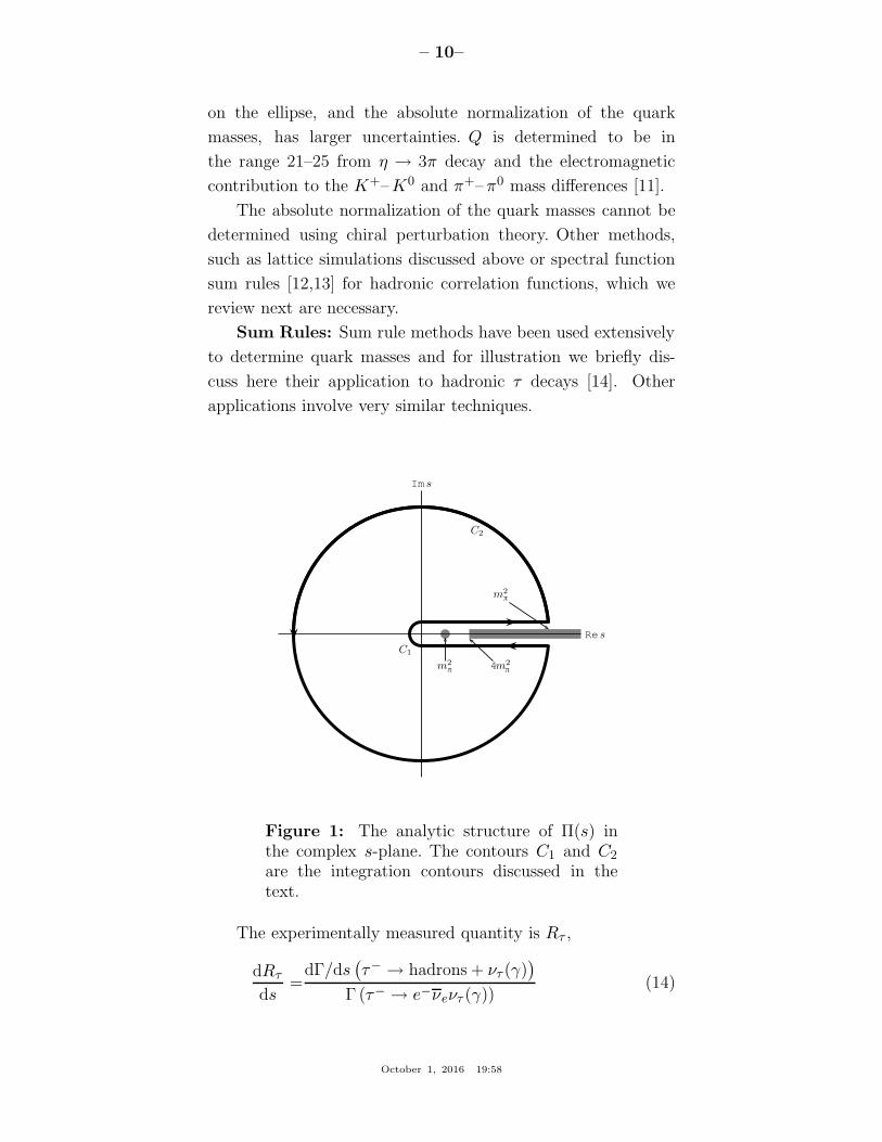
Figure 1: The analytic structure of Π(s) inthe complex s-plane. The contours C1 and C2

are the integration contours discussed in thetext.

The experimentally measured quantity is Rτ ,

dRτ

ds=

dΓ/ds(

τ− → hadrons + ντ (γ))

Γ (τ− → e−νeντ (γ))(14)

October 1, 2016 19:58

– 11–

the hadronic invariant mass spectrum in semihadronic τ decay,

normalized to the leptonic τ decay rate. It is useful to define q

as the total momentum of the hadronic final state, so s = q2 is

the hadronic invariant mass. The total hadronic τ decay rate

Rτ is then given by integrating dRτ/ds over the kinematically

allowed range 0 ≤ s ≤ M2τ .

Rτ can be written as

Rτ =12π

∫ M2τ

0

ds

M2τ

(

1 −s

M2τ

)2

×

[(

1 + 2s

M2τ

)

Im ΠT (s) + Im ΠL(s)

]

(15)

where s = q2, and the hadronic spectral functions ΠL,T are

defined from the time-ordered correlation function of two weak

currents is the time-ordered correlator of the weak interaction

current (jµ(x) and jν(0)) by

Πµν(q) =i

∫

d4x eiq·x 〈0|T(

jµ(x)jν(0)†)

|0〉 , (16)

Πµν(q) = (−gµν + qµqν)ΠT (s) + qµqνΠL(s), (17)

and the decomposition Eq. (17) is the most general possible

structure consistent with Lorentz invariance.

By the optical theorem, the imaginary part of Πµν is

proportional to the total cross-section for the current to produce

all possible states. A detailed analysis including the phase space

factors leads to Eq. (15). The spectral functions ΠL,T (s) are

analytic in the complex s plane, with singularities along the real

axis. There is an isolated pole at s = m2π, and single- and multi-

particle singularities for s ≥ 4m2π, the two-particle threshold.

The discontinuity along the real axis is ΠL,T (s+i0+)−ΠL,T (s−

i0+) = 2iIm ΠL,T (s). As a result, Eq. (15) can be rewritten

with the replacement Im ΠL,T (s) → −iΠL,T (s)/2, and the

integration being over the contour C1. Finally, the contour C1

can be deformed to C2 without crossing any singularities, and

so leaving the integral unchanged. One can derive a series of

sum rules analogous to Eq. (15) by weighting the differential τ

October 1, 2016 19:58

– 12–

hadronic decay rate by different powers of the hadronic invariant

mass,

Rklτ =

∫ M2τ

0

ds

(

1 −s

M2τ

)k (

s

M2τ

)ldRτ

ds(18)

where dRτ/ds is the hadronic invariant mass distribution in τ

decay normalized to the leptonic decay rate. This leads to the

final form of the sum rule(s),

Rklτ = − 6πi

∫

C2

ds

M2τ

(

1 −s

M2τ

)2+k (

s

M2τ

)l

×

[(

1 + 2s

M2τ

)

ΠT (s) + ΠL(s)

]

. (19)

The manipulations so far are completely rigorous and exact,

relying only on the general analytic structure of quantum field

theory. The left-hand side of the sum rule Eq. (19) is obtained

from experiment. The right hand-side can be computed for s

far away from any physical cuts using the operator product

expansion (OPE) for the time-ordered product of currents

in Eq. (16), and QCD perturbation theory. The OPE is an

expansion for the time-ordered product Eq. (16) in a series of

local operators, and is an expansion about the q → ∞ limit. It

gives Π(s) as an expansion in powers of αs(s) and Λ2QCD/s, and

is valid when s is far (in units of Λ2QCD) from any singularities

in the complex s-plane.

The OPE gives Π(s) as a series in αs, quark masses, and

various non-perturbative vacuum matrix element. By comput-

ing Π(s) theoretically, and comparing with the experimental

values of Rklτ , one determines various parameters such as αs

and the quark masses. The theoretical uncertainties in using

Eq. (19) arise from neglected higher order corrections (both

perturbative and non-perturbative), and because the OPE is

no longer valid near the real axis, where Π has singularities.

The contribution of neglected higher order corrections can be

estimated as for any other perturbative computation. The error

due to the failure of the OPE is more difficult to estimate. In

Eq. (19), the OPE fails on the endpoints of C2 that touch the

real axis at s = M2τ . The weight factor (1 − s/M2

τ ) in Eq. (19)

October 1, 2016 19:58

– 13–

vanishes at this point, so the importance of the endpoint can

be reduced by choosing larger values of k.

E. Heavy quarks

For heavy-quark physics one can exploit the fact that

mQ ≫ ΛQCD to construct effective theories (mQ is the mass of

the heavy quark Q). The masses and decay rates of hadrons

containing a single heavy quark, such as the B and D mesons

can be determined using the heavy quark effective theory

(HQET) [45]. The theoretical calculations involve radiative

corrections computed in perturbation theory with an expansion

in αs(mQ) and non-perturbative corrections with an expansion

in powers of ΛQCD/mQ. Due to the asymptotic nature of the

QCD perturbation series, the two kinds of corrections are

intimately related; an example of this are renormalon effects

in the perturbative expansion which are associated with non-

perturbative corrections.

Systems containing two heavy quarks such as the Υ or

J/Ψ are treated using non-relativistic QCD (NRQCD) [46].

The typical momentum and energy transfers in these systems

are αsmQ, and α2smQ, respectively, so these bound states are

sensitive to scales much smaller than mQ. However, smeared

observables, such as the cross-section for e+e− → bb averaged

over some range of s that includes several bound state energy

levels, are better behaved and only sensitive to scales near mQ.

For this reason, most determinations of the c, b quark masses

using perturbative calculations compare smeared observables

with experiment [47–49].

There are many continuum extractions of the c and b quark

masses, some with quoted errors of 10 MeV or smaller. There

are systematic effects of comparable size, which are typically not

included in these error estimates. Reference [41], for example,

shows that even though the error estimate of mc using the rapid

convergence of the αs perturbation series is only a few MeV,

the central value of mc can differ by a much larger amount

depending on which algorithm (all of which are formally equally

good) is used to determine mc from the data. This leads to a

systematic error from perturbation theory of around 20 MeV

for the c quark and 25 MeV for the b quark. Electromagnetic

October 1, 2016 19:58

– 14–

effects, which also are important at this precision, are often

not included. For this reason, we inflate the errors on the

continuum extractions of mc and mb. The average values of mc

and mb from continuum determinations are (see Sec. G for the

1S scheme)

mc(mc) = (1.28 ± 0.025) GeV

mb(mb) = (4.18 ± 0.03) GeV , m1Sb = (4.65 ± 0.03) GeV .

Lattice simulations of QCD lead to discretization errors

which are powers of mQ a (modulated by logarithms); the

power depends on the formulation of lattice QCD being used

and in most cases is quadratic. Clearly these errors can be re-

duced by performing simulations at smaller lattice spacings, but

also by using improved discretizations of the theory. Recently,

with more powerful computing resources, better algorithms and

techniques, it has become possible to perform simulations in

the charm quark region and beyond, also decreasing the ex-

trapolation which has to be performed to reach the b-quark. A

novel approach proposed in [64] has been to compare the lattice

results for moments of correlation functions of cc quark-bilinear

operators to perturbative calculations of the same quantities

at 4-loop order. In this way both the strong coupling constant

and the charm quark mass can be determined with remark-

ably small errors; in particular mc(mc) = 1.273(6) GeV [36].

This lattice determination also uses the perturbative expression

for the current-current correlator, and so has the perturbation

theory systematic error discussed above. Recent updates using

this correlator method, both with a very similar result, can be

found in [27,37]. It should be remembered that these results

were obtained in QCD with exact isospin symmetry; isospin

breaking effects, including electromagnetism may well be larger

or of the order of the quoted uncertainty.

As the range of heavy-quark masses which can be used in

numerical simulations increases, results obtained by extrapo-

lating the results to b-physics are becoming ever more reliable

(see e.g. [27]) . Traditionally however, the main approach to

controlling the discretization errors in lattice studies of heavy

quark physics has been to perform simulations of the effective

October 1, 2016 19:58

– 15–

theories such as HQET and NRQCD. This remains an impor-

tant technique, both in its own right and in providing additional

information for extrapolations from lower masses to the bottom

region. Using effective theories, mb is obtained from what is

essentially a computation of the difference of MHb− mb, where

MHbis the mass of a hadron Hb containing a b-quark. The

relative error on mb is therefore much smaller than that for

MHb− mb. The principal systematic errors are the matching

of the effective theories to QCD and the presence of power

divergences in a−1 in the 1/mb corrections which have to be

subtracted numerically. The use of HQET or NRQCD is less

precise for the charm quark, but in this case, as mentioned

above, direct QCD simulations are now possible.

F. Pole Mass

For an observable particle such as the electron, the position

of the pole in the propagator is the definition of its mass.

In QCD this definition of the quark mass is known as the

pole mass. It is known that the on-shell quark propagator has

no infrared divergences in perturbation theory [52,53], so

this provides a perturbative definition of the quark mass. The

pole mass cannot be used to arbitrarily high accuracy because

of nonperturbative infrared effects in QCD. The full quark

propagator has no pole because the quarks are confined, so that

the pole mass cannot be defined outside of perturbation theory.

The relation between the pole mass mQ and the MS mass mQ

is known to three loops [54,55,56,57]

mQ = mQ(mQ)

{

1 +4αs(mQ)

3π

+

[

−1.0414∑

k

(

1 −4

3

mQk

mQ

)

+ 13.4434

]

[

αs(mQ)

π

]2

+[

0.6527N2L − 26.655NL + 190.595

]

[

αs(mQ)

π

]3}

, (20)

where αs(µ) is the strong interaction coupling constants in the

MS scheme, and the sum over k extends over the NL flavors Qk

lighter than Q. The complete mass dependence of the α2s term

October 1, 2016 19:58

– 16–

can be found in [54]; the mass dependence of the α3s term is

not known. For the b-quark, Eq. (20) reads

mb = mb (mb) [1 + 0.10 + 0.05 + 0.03] , (21)

where the contributions from the different orders in αs are shown

explicitly. The two and three loop corrections are comparable

in size and have the same sign as the one loop term. This is

a signal of the asymptotic nature of the perturbation series

[there is a renormalon in the pole mass]. Such a badly behaved

perturbation expansion can be avoided by directly extracting

the MS mass from data without extracting the pole mass as an

intermediate step.

G. Numerical values and caveats

The quark masses in the particle data listings have been

obtained by using a wide variety of methods. Each method

involves its own set of approximations and uncertainties. In

most cases, the errors are an estimate of the size of neglected

higher-order corrections or other uncertainties. The expansion

parameters for some of the approximations are not very small

(for example, they are m2K/Λ2

χ ∼ 0.25 for the chiral expansion

and ΛQCD/mb ∼ 0.1 for the heavy-quark expansion), so an

unexpectedly large coefficient in a neglected higher-order term

could significantly alter the results. It is also important to note

that the quark mass values can be significantly different in the

different schemes.

The heavy quark masses obtained using HQET, QCD sum

rules, or lattice gauge theory are consistent with each other

if they are all converted into the same scheme and scale. We

have specified all masses in the MS scheme. For light quarks,

the renormalization scale has been chosen to be µ = 2GeV.

The light quark masses at 1GeV are significantly different from

those at 2GeV, m(1 GeV)/m(2 GeV) ∼ 1.33. It is conventional

to choose the renormalization scale equal to the quark mass for

a heavy quark, so we have quoted mQ(µ) at µ = mQ for the c

and b quarks. Recent analyses of inclusive B meson decays have

shown that recently proposed mass definitions lead to a better

behaved perturbation series than for the MS mass, and hence to

more accurate mass values. We have chosen to also give values

October 1, 2016 19:58

– 17–

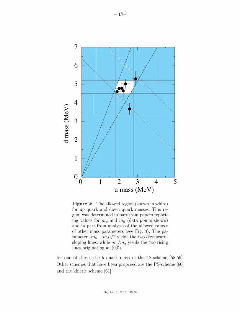
Figure 2: The allowed region (shown in white)for up quark and down quark masses. This re-gion was determined in part from papers report-ing values for mu and md (data points shown)and in part from analysis of the allowed rangesof other mass parameters (see Fig. 3). The pa-rameter (mu + md)/2 yields the two downward-sloping lines, while mu/md yields the two risinglines originating at (0,0).

for one of these, the b quark mass in the 1S-scheme [58,59].

Other schemes that have been proposed are the PS-scheme [60]

and the kinetic scheme [61].

October 1, 2016 19:58

– 18–

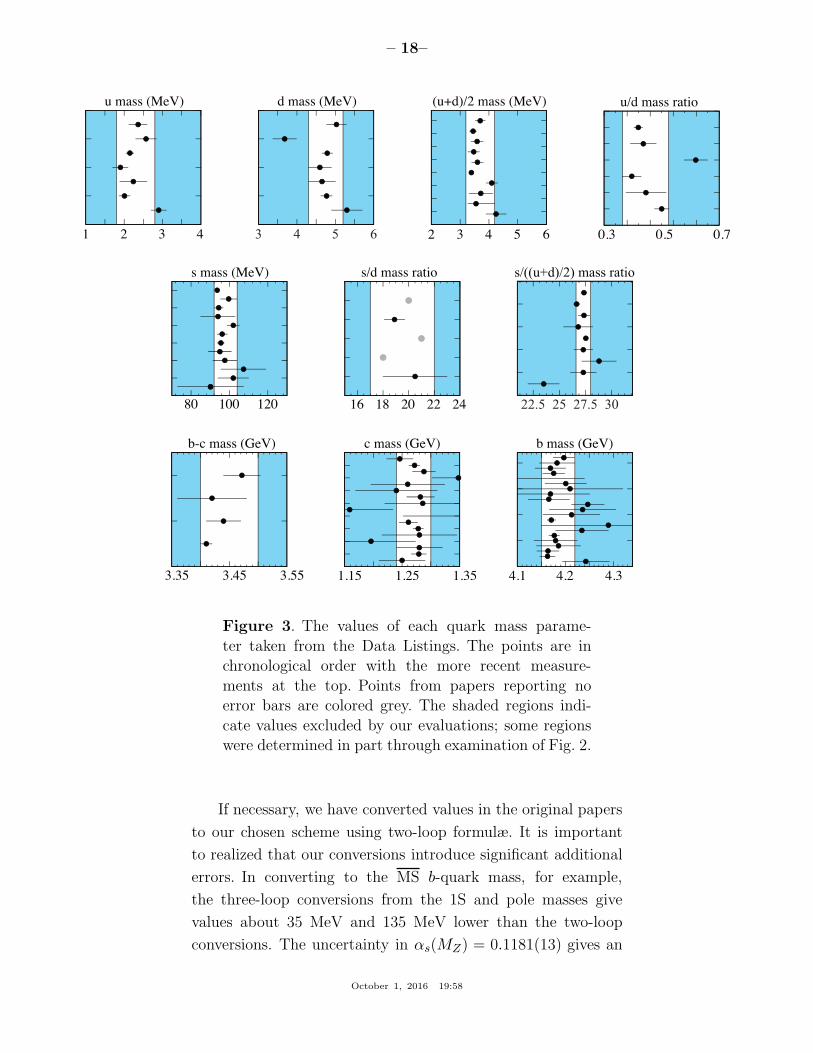
Figure 3. The values of each quark mass parame-

ter taken from the Data Listings. The points are inchronological order with the more recent measure-

ments at the top. Points from papers reporting noerror bars are colored grey. The shaded regions indi-

cate values excluded by our evaluations; some regionswere determined in part through examination of Fig. 2.

If necessary, we have converted values in the original papers

to our chosen scheme using two-loop formulæ. It is important

to realized that our conversions introduce significant additional

errors. In converting to the MS b-quark mass, for example,

the three-loop conversions from the 1S and pole masses give

values about 35 MeV and 135 MeV lower than the two-loop

conversions. The uncertainty in αs(MZ) = 0.1181(13) gives an

October 1, 2016 19:58

– 19–

uncertainty of ±10 MeV and ±35 MeV respectively in the same

conversions. We have not added these additional errors when we

do our conversions. The αs value in the conversion is correlated

with the αs value used in determining the quark mass, so the

conversion error is not a simple additional error on the quark

mass.

References

1. See the review of QCD in this volume..

2. A.V. Manohar and H. Georgi, Nucl. Phys. B234, 189(1984).

3. K.G. Chetyrkin, Phys. Lett. B404, 161 (1997).

4. J.A.M. Vermaseren, S.A. Larin, and T. van Ritbergen,Phys. Lett. B405, 327 (1997).

5. K.G. Chetyrkin, B.A. Kniehl, and M. Steinhauser, Nucl.Phys. B510, 61 (1998).

6. S. Weinberg, Physica 96A, 327 (1979).

7. J. Gasser and H. Leutwyler, Ann. Phys. 158, 142 (1984).

8. For a review, see A. Pich, Rept. on Prog. in Phys. 58, 563(1995).

9. S. Weinberg, Trans. N.Y. Acad. Sci. 38, 185 (1977).

10. D.B. Kaplan and A.V. Manohar, Phys. Rev. Lett. 56,2004 (1986).

11. H. Leutwyler, Phys. Lett. B374, 163 (1996).

12. S. Weinberg, Phys. Rev. Lett. 18, 507 (1967).

13. M.A. Shifman, A.I. Vainshtein, and V.I. Zakharov, Nucl.Phys. B147, 385 (1979).

14. E. Braaten, S. Narison, and A. Pich, Nucl. Phys. B373,581 (1992).

15. C. Bernard et al., PoS LAT2007 (2007) 090.

16. S. Aoki et al. [FLAG Collab.], Eur. Phys. J. C74, 2890(2014).

17. A. Bazavov et al., arXiv:0903.3598 [hep-lat].

18. C. Aubin et al. [HPQCD Collab.], Phys. Rev. D70, 031504(2004).

19. C. Aubin et al. [MILC Collab.], Phys. Rev. D70, 114501(2004).

20. B. Blossier et al. [ETM Collab.], Phys. Rev. D82, 114513(2010).

21. A. Bazavov et al. [MILC Collab.], PoS CD09 (2009) 007.

October 1, 2016 19:58

– 20–

22. A. Bazavov et al., PoS LATTICE2010 (2010) 083.

23. S. Durr et al., Phys. Lett. B701, 265 (2011).

24. S. Durr et al., J. High Energy Phys.1108,148(2011).

25. R. Arthur et al. [RBC and UKQCD Collabs.], Phys. Rev.D87, 094514 (2013).

26. A. Bazavov et al. [Fermilab Lattice and MILC Collabs.],Phys. Rev. D90, 074509 (2014).

27. B. Chakraborty et al., Phys. Rev. D91, 054508 (2015).

28. N. Carrasco et al. [European Twisted Mass Collab.], Nucl.Phys. B887, 19 (2014).

29. “Domain wall QCD with physical quark masses,” T. Blumet al. [RBC and UKQCD Collabs.], arXiv:1411.7017

[hep-lat].

30. S. Borsanyi et al., Science 347, 1452 (2015).

31. Y. Aoki et al. [RBC and UKQCD Collabs.], Phys. Rev.D83, 074508 (2011).

32. S. Basak et al. [MILC Collab.], J. Phys. Conf. Ser. 640

(2015) 1, 012052.

33. T. Blum et al., Phys. Rev. D82, 094508 (2010).

34. S. Aoki et al., Phys. Rev. D86, 034507 (2012).

35. C.T.H. Davies et al., Phys. Rev. Lett. 104, 132003 (2010).

36. C. McNeile et al., Phys. Rev. D82, 034512 (2010).

37. K. Nakayama, B. Fahy, and S. Hashimoto, arXiv:1511.09163[hep-lat]..

38. C. Aubin et al. [MILC Collab.], Nucl. Phys. (Proc. Supp.)140, 231 (2005).

39. C. Aubin et al. [MILC Collab.], Phys. Rev. D70, 114501(2004).

40. G. Colangelo et al., Eur. Phys. J. C71, 1695 (2011).

41. B. Dehnadi et al., arXiv:1102.2264 [hep-ph].

42. T. Blum et al., Phys. Rev. D76, 114508 (2007).

43. G. Colangelo et al., Eur. Phys. J. C71, 1695 (2011).

44. A. Ali Khan et al. [CP-PACS Collab.], Phys. Rev. D65,054505 (2002); [Erratum-ibid. D 67 (2003) 059901].

45. N. Isgur and M.B. Wise, Phys. Lett. B232, 113 (1989),ibid, B237, 527 (1990).

46. G.T. Bodwin, E. Braaten, and G.P. Lepage, Phys. Rev.D51, 1125 (1995).

47. A.H. Hoang, Phys. Rev. D61, 034005 (2000).

48. K. Melnikov and A. Yelkhovsky, Phys. Rev. D59, 114009(1999).

October 1, 2016 19:58

– 21–

49. M. Beneke and A. Signer, Phys. Lett. B471, 233 (1999).

50. A.X. El-Khadra, A.S. Kronfeld, and P.B. Mackenzie, Phys.Rev. D55, 3933 (1997).

51. S. Aoki, Y. Kuramashi, and S.i. Tominaga, Prog. Theor.Phys. 109, 383 (2003).

52. R. Tarrach, Nucl. Phys. B183, 384 (1981).

53. A. Kronfeld, Phys. Rev. D58, 051501 (1998).

54. N. Gray et al., Z. Phys. C48, 673 (1990).

55. D.J. Broadhurst, N. Gray, and K. Schilcher, Z. Phys. C52,111 (1991).

56. K.G. Chetyrkin and M. Steinhauser, Phys. Rev. Lett. 83,4001 (1999).

57. K. Melnikov and T. van Ritbergen, Phys. Lett. B482, 99(2000).

58. A.H. Hoang, Z. Ligeti, A.V. Manohar, Phys. Rev. Lett.82, 277 (1999).

59. A.H. Hoang, Z. Ligeti, A.V. Manohar, Phys. Rev. D59,074017 (1999).

60. M. Beneke, Phys. Lett. B434, 115 (1998).

61. P. Gambino and N. Uraltsev, Eur. Phys. J. C34, 181(2004).

62. G. Martinelli et al., Nucl. Phys. B445, 81 (1995).

63. K. Jansen et al., Phys. Lett. B372, 275 (1996).

64. I. Allison et al. [HPQCD Collab.], Phys. Rev. D78, 054513(2008).

October 1, 2016 19:58