1

Performance Analysis of FDD Massive MIMO

Systems under Channel Aging

Ribhu Chopra, Member, IEEE, Chandra R. Murthy, Senior Member, IEEE, Himal

A. Suraweera, Senior Member, IEEE, and Erik G. Larsson, Fellow, IEEE

Abstract

In this paper, we study the effect of channel aging on the uplink and downlink performance of

an FDD massive MIMO system, as the system dimension increases. Since the training duration scales

linearly with the number of transmit dimensions, channel estimates become increasingly outdated in

the communication phase, leading to performance degradation. To quantify this degradation, we first

derive bounds on the mean squared channel estimation error. We use the bounds to derive deterministic

equivalents of the receive SINRs, which yields a lower bound on the achievable uplink and downlink

spectral efficiencies. For the uplink, we consider maximal ratio combining and MMSE detectors, while

for the downlink, we consider matched filter and regularized zero forcing (RZF) precoders. We show

that the effect of channel aging can be mitigated by optimally choosing the frame duration. It is found

that using all the base station antennas can lead to negligibly small achievable rates in high user

mobility scenarios. Finally, numerical results are presented to validate the accuracy of our expressions

and illustrate the dependence of the performance on the system dimension and channel aging parameters.

Index Terms

Massive MIMO, channel aging, channel estimation, performance analysis, achievable rate.

R. Chopra is with the Department of Electronics and Electrical Engineering, Indian Institute of Technology Guwahati, Assam,India. (email: ribhufec@iitg.ernet.in).

C. R. Murthy is with the Department of Electrical Communication Engineering, Indian Institute of Science, Bangalore, India.(email: cmurthy@ece.iisc.ernet.in).

H. A. Suraweera is with the Department of Electrical and Electronic Engineering, University of Peradeniya, Peradeniya, SriLanka (email: himal@ee.pdn.ac.lk).

E. G. Larsson is with the Department of Electrical Engineering (ISY), Linkoping University, Sweden (email:erik.g.larsson@liu.se).

2

I. INTRODUCTION

Multiple-input multiple-output (MIMO) with a large number of base station antennas serving

multiple users, popularly known as massive MIMO, is a key enabling technology for next gen-

eration wireless communications [1]–[3]. A singular feature of these systems is the phenomenon

of channel hardening due to large dimensions [4], that leads to quasi orthogonality among

different channel vectors [5]–[7]. This quasi-orthogonality reduces the inter-stream interference,

allowing the use of simplified transmitter and receiver architectures. Further, the array gain

increases linearly with the number of base station antennas [7], [8], leading to increased spectral

and energy efficiencies. However, the above advantages of massive MIMO rely heavily on the

availability of accurate and up to date channel state information (CSI) at the base station and

the users. In practice, the CSI at the base station is imperfect because of channel estimation

errors [9]–[11], pilot contamination [10] and is also outdated due to channel aging [12].

Channel aging is caused by the time varying nature of the channel between the cellular users

and the base station, which is in turn a consequence of user mobility [12], [13]. Contrary to

the conventional block fading channel model, an aging channel evolves continuously with time,

and is different during each transmitted symbol. This results in a mismatch between the actual

channel state and the CSI acquired during training, which could degrade the performance of a

massive MIMO system [13]. More importantly, since the minimum training duration for acquiring

CSI scales linearly with the number of antennas, the mismatch gets exacerbated with increasing

system dimensionality. As a consequence, having more antennas at the base station may in fact

lead to poor performance in the presence of channel aging.

Most of the current literature [12]–[17], starting from [12], focuses on the effects of channel

aging for time division duplexed (TDD) massive MIMO systems. In general, and the performance

loss due to channel aging is quantified using the achievable rate of the system under study. All

of the present works on channel aging consider linear receivers such as the maximal ratio

combining (MRC) receiver [12] and the minimum mean squared error (MMSE) receiver [14]

in the uplink, and linear precoders such as the matched filter precoder (MFP) [12] and the

regularized zero forcing (RZF) [13] precoder in the downlink. Linear receivers and precoders

are mainly chosen due to their simplicity and ease of analysis. The achievable rates have generally

been derived using a deterministic equivalent (DE) of the signal to interference plus noise

3

ratios (SINRs), and then using the DE-SINR to compute the achievable rates. The authors in [13]

also derive the non asymptotic achievable rates in addition to the more conventional DE analysis.

The results derived in these papers confirm that although the benefits of massive MIMO such

as power scaling [18] are still valid in the presence of channel aging, it does indeed lead to

a significant loss in the user performance, and its effect is accentuated by an increase in user

mobility [19]. The effect of channel aging on TDD massive MIMO systems have been also been

studied in conjunction with phase noise [13] and pilot contamination [20].

However, the extension of current massive MIMO techniques to an FDD setting has been

identified as an open challenge in [18]. The study of the effect of channel aging in an FDD

setting is also important because it is easier for the current cellular systems to upgrade to

massive MIMO in an FDD system, rather than switch to TDD [18], [21], [22]. Transmission

schemes and channel estimation for FDD based massive MIMO have been discussed in [23]

and [21], respectively. Contrary to the TDD massive MIMO model, channel reciprocity cannot

be assumed in an FDD massive MIMO system. Consequently, forward link training is required

for both uplink and downlink, making the problem of channel aging more pronounced when the

base station is equipped with a large number of antennas. The effect of channel aging on the

downlink of a beamforming based single user large MIMO system has been examined in [24].

In [24], the minimum achievable rate is optimized in terms of the number of transmit antennas

and the frame duration. It is shown that, it is not always beneficial to use a larger number of

base station antennas, and the overall throughput of such a system may degrade with an increase

in the number of transmit antennas.

Most of the current literature on the effects of channel aging on massive MIMO systems

assumes no variation in the channel during the training interval [12]–[14], [16]. While this

assumption simplifies the determination of channel estimation error variances, that are needed

to compute the achievable rates for different systems, it is unrealistic since the channel will

continue to age during the training phase, and the quality of estimates of different users will be

different due to their different training instants. Kalman filter based estimators for aging channels

have been derived in [25] but the effects of estimation errors on the achievable data rates have

not been discussed.

In this paper, we consider linear channel estimation, precoding, and receive combining, in a

single cell multiuser FDD massive MIMO setting. We first characterize the performance of the

4

MMSE channel estimators for both the uplink and downlink channels, and derive bounds on the

quality of the channel estimates at the end of the training duration. We then use these results to

obtain lower bounds on the achievable rate in both uplink and downlink. We study the behavior

of the MRC and the MMSE receivers for the uplink, and the MF and the RZF precoders in the

downlink. The main contributions of this work can be listed as follows:

1) We derive bounds on the mean squared channel estimation error for both the uplink and the

downlink channels, accounting for the effect of channel aging during the training interval.

We observe that the performance of channel estimation saturates in the presence of channel

aging, and the saturated value of the MSE normalized with respect to the mean squared

channel gain for downlink channel estimation can be as large as −3 dB for user velocities

of the order of 100 km/h. (See Section III.)

2) We use DE analysis along with the derived bounds on the channel estimation errors to

characterize the per user achievable rates in the uplink for the MRC and the MMSE

receivers. Increased user mobilities are observed to reduce the achievable rate by more

than a factor of two in an MMSE receiver based system with 150 cellular users. (See

Section IV.)

3) We derive the DEs of the per user achievable rate in the downlink for the MFP and RZF

precoders using the bounds on the mean squared channel estimation errors, and show that

using a larger number of transmit antennas may not lead to improved data rates under

channel aging conditions. For example, in a 100 user system with a base station equipped

with 1000 antennas, using all the antennas at user velocities beyond 200 km/h may lead

to a negligibly small achievable rate, even after optimizing the frame duration based on

the channel aging parameters. (See Section IV.)

4) Via detailed simulations, we prescribe the optimal values of different parameters such as

frame duration, number of base station antennas used, etc. under different channel aging

conditions. We observe that the optimal frame duration for a system with high user mobility

is a function of the number of users.

The key findings of this work are that channel aging severely affects both channel estimation

and achievable rates in an FDD massive MIMO system. It is therefore not always better to use

a larger number of antennas at the base station. We have thus identified new tradeoffs due to

5

Fig. 1: The system model.

channel aging that need to be taken into account while designing massive MIMO systems.

II. TIME VARYING CHANNEL MODEL

Our system model, as illustrated in Fig. 1, considers a single cell system with a base station

having N antennas communicating with K < N single antenna users indexed by k ∈ {1, . . . , K}.

We assume an FDD system with training for channel estimation in both the uplink and the

downlink. In the uplink frame, each user first transmits orthogonal pilot symbols to the base

station, where these are used to estimate the underlying channels. Following this, all the users

simultaneously transmit their data to the base station. The data is detected at the base station

using the CSI acquired during the pilot transmission phase. During the downlink training phase,

the base station transmits orthogonal pilot symbols from its antennas which are used by the users

to estimate the corresponding downlink channel. These channel estimates are then fed back to

the base station by the users, and are used by the latter to appropriately precode the data symbols

transmitted simultaneously to all the users during the data transmission phase. We assume an

ideal delay and error free feedback channel for ease of analysis and also to isolate the effect of

channel aging and estimation error on the system performance.

The uplink channel between the kth user and the ith base station antenna at the nth instant

is modeled as√βkhik[n], with βk representing the (large scale) slow fading and path loss

component, and hik[n] representing the fast fading component modeled as a zero mean circularly

6

symmetric complex Gaussian (ZMCSCG) random variable (rv) with unit variance, denoted

by CN (0, 1). Similarly, the downlink channel from the ith base station antenna to the kth user

can be expressed as√βkfki[n] with fki[n] representing the CN (0, 1) distributed fast fading

component. Note that the slow fading and path loss component is assumed to be the same in

the uplink and downlink channels, and the same across all base station antennas.

Defining β = [β1, . . . , βK ]T , we can write the uplink channel matrix at the nth instant as

H[n]diag(√β), with H[n] ∈ CN×K , with the entries of H[n] being CN (0, 1), and diag(β)

representing a K × K diagonal matrix such that (diag(β))kk = βk. Similarly, the downlink

channel is expressed as diag(√β)F[n] with F[n] ∈ CK×N .

The temporal variations in the propagation environment, caused due to user mobility, results in

the channel coefficients evolving with time. The channel evolution can be modeled as a function

of its initial state and an innovation component, such that the channel between the ith base

station antenna and the kth user at the nth instant is [12], [26]

hik[n] = ρ[n]hik[0] + ρ[n]zh,ik[n]

fki[n] = ρ[n]fki[0] + ρ[n]zf,ki[n], (1)

where zh,ik[n] ∼ CN (0, 1) and zf,ki[n] ∼ CN (0, 1) are respectively the innovation components

for the uplink and downlink channels, 0 ≤ ρ[n] ≤ 1 is the correlation between the channel

instances at lags 0 and n, and ρ[n] =√

1− |ρ[n]|2. The channel innovation processes, zh,ik[n]

and zf,ki[n], need not be temporally white. Their statistics are chosen such that the second-order

statistics of the model in (1) match with the temporal correlation of the channel. Specifically,

if Ch denotes the temporal covariance matrix of the instances of one of the channel entries at

times 1 through (T −1), the (T −1)×(T −1) covariance Rz of an entry of the innovation vector

sequence is given by Rz = D−1(Ch− ρ ρT )D−1, where ρ , [ρ[1], ρ[2], . . . , ρ[T − 1]]T and D ,

diag(ρ[1], . . . , ρ[T − 1]). Since channel aging is mainly caused due to relative motion between

the transmitter and the receiver, the temporal channel correlation coefficient can be assumed

to be the same for the uplink and the downlink channels. It is conventional to assume that the

channel evolves according to the Jakes’ model [12], [27], or as a first order autoregressive (AR1)

process [24]. If the channel is assumed to age according to the Jakes’ model [27], ρ[n] =

J0(2πfdTsn), where fd is the Doppler frequency, Ts is the sampling period, and J0(·) is the

7

Bessel function of the first kind and zeroth order [28, Eq. (9.1.18)]. Also, each entry of the

channel vector is temporally as [Ch]mk = J0(2π(m − k)fdTS). Alternatively, if we consider

the channel to evolve as an AR1 model, ρ[n] = ρn, with ρ being J0(2πfdTs), and Ch is

a symmetric Toeplitz matrix with [1, ρ, ρ2, . . . , ρT−1] as its first row. We assume ρ[n] to be

identical across all users for simplicity. Note that, the model in (1) differs from the AR1 model

(or more generally, the AR(p) model) commonly used in the literature in that the channel state

is determined recursively in terms of its state at the previous time instant, instead of its state

at an initial time hik[0]. Furthermore, the coefficients of the AR(p) model are chosen such that

the statistics of the channel approximately match with that of the Jakes’ model. This is an

advantage of the model in (1), namely, that the statistics of the innovation processes can be

chosen such that the statistics of the model exactly match with that of the Jakes’ model within

a finite-time window of interest. Also, since the effects of phase noise discussed in [13] can be

incorporated into the channel autocorrelation function, we do not discuss these explicitly, and

use a generalized correlation coefficient ρ[n].

III. CHANNEL ESTIMATION

In this section, we consider MMSE estimation of the uplink and the downlink channels,

and provide expressions for the MSE for channel estimation in both the cases. We use these

expressions to show that the performance of the estimator saturates due to channel aging.

A. Uplink Channels

Since there are K users transmitting to an N antenna base station in the uplink, the minimal

number of uplink pilot symbols for channel estimation at the base station is K [29]. Hence, the

signal received at the ith base station antenna at the nth instant can be written as,

yi[n] =K∑k=1

√βkEu,p,khik[n]ψk[n] +

√N0wi[n], (2)

where Eu,p,k is the pilot energy of the kth user, N0 is the noise variance, and wi[0] ∼ CN (0, 1).

The quality of the channel estimate will worsen with an increase in the delay between training

and transmission, hence, we consider the channel estimates at n = K+1, as the channel estimates

at later instants will only be worse. The effective channel at the nth (n ≤ K) instant can be

8

expressed in terms of the channel at the (K + 1)th instant as

hik[n] = ρ∗[K + 1− n]hik[K + 1] + ρ[K + 1− n]ζh,ik[n]. (3)

Consequently, (2) can be rewritten as

yi[n] =K∑m=1

√βmEu,p,mρ∗[K + 1− n]ψm[n]him[K + 1]

+K∑m=1

√βmEu,p,mρ[K + 1− n]ψm[n]ζh,im[n] +

√N0wi[n], (4)

with ψm[n] corresponding to the pilot signal transmitted by the mth user at the nth time instant.

For channel estimation, we consider a weighted combination of the received training signals

with weights ck[n] chosen to match with the training sequences, ψm[n] attenuated by the aging

component, i.e.,K∑n=1

ck[n]ρ∗[K + 1− n]ψm[n] = δ[k −m], (5)

where δ[·] is the Kronecker delta function. Thus, the combined received signal can be written as

uik =K∑m=1

√βmEu,p,mhim[K + 1]

K∑n=1

ρ∗[K + 1− n]ck[n]ψm[n]

+K∑m=1

√βmEu,p,m

K∑n=1

ρ[K + 1− n]ck[n]ψm[n]ζh,im[n] +√N0

K∑n=1

ck[n]wi[n]. (6)

If ck[n] and ψm[n] satisfy the orthogonality condition in (5), which is a commonly used design

criterion in pilot design for channel estimation, and further letting ψm[n] = δ[n − m] and

ck[n] = (ρ∗[K − n])−1δ[n− k] (which satisfies (5)), we get

uik =√βkEu,p,khik[K + 1] +

√βkEu,p,kρ−1∗[K + 1− k]ρ[K + 1− k]ζh,ik[k]

+ρ−1∗[K + 1− k]√N0wi[k]. (7)

In the above, the first term corresponds to the channel coefficient of interest, and the others

are additive noise terms. Since the coefficients hik[K + 1] are i.i.d., they can be individually

9

estimated from the corresponding uik. The MMSE estimate, hik of hik[K + 1] is given by

hik = ρ[K + 1− k]

√1

βkEu,p,k +N0

uik. (8)

Therefore, the estimation error variance, denoted as σ2h,ik, becomes

σ2h,ik =

|ρ[K + 1− k]|2βkEu,p,k +N0

βkEu,p,k +N0

. (9)

Now, σ2h,ik can be bounded as

|ρ[1]|2βkEu,p,k +N0

βkEu,p,k +N0

≤ σ2h,ik ≤

|ρ[K]|2βkEu,p,k +N0

βkEu,p,k +N0

. (10)

This holds for all sequences ck[n] and ψm[n] satisfying the orthogonality condition (5).

Letting γu,p,k ,βkEu,p,kN0

, we can write an upper bound on the MSE for channel estimation as

σ2h,ik ≤

|ρ[K]|2γu,p,k + 1

γu,p,k + 1. (11)

Now, looking at the MSE in the absence of channel aging, σ′2h,ik = 1γu,p,k+1

, we observe that in the

absence of channel aging, the estimation error disappears as the pilot signal-to-noise ratio (SNR),

γu,p,k grows. However, in the presence of channel aging from (9),

limγu,p,k→∞

σ2h,ik = |ρ[K + 1− k]|2. (12)

That is, the channel estimation error saturates, and the limiting MSE worsens as the number

of users increases. Thus, aging adversely affects the quality of the channel estimates. We next

discuss the effects of aging on downlink channel estimation.

B. Downlink Channels

Similar to the uplink, the N antennas at the base station transmit a pilot sequence {ψ[n]}Nn=1

with energies Ed,p. The signal received at the kth user at the nth instant is

yk[n] =N∑i=1

√βkEd,pfki[n]ψi[n] +

√N0wk[n], (13)

where ψi[n] is the pilot symbol transmitted by the ith base station antenna at the nth instant. We

are interested in estimating the channel between the kth user and the ith base station antenna,

10

which is related to the channel at the nth instant, fki[n], via fki[n] = ρ∗[N + 1− n]fki[N + 1] +

ρ[N + 1− n]ζd,ki[n]. Therefore,

yk[n] =N∑i=1

√βkEd,p(ρ∗[N + 1 − n]fki[N + 1] + ρ[N + 1 − n]ζd,ki[n])ψi[n] +

√N0wk[n].

Defining uki ,∑N

n=1 ci[n]yk[n], where ci[n] is chosen such that∑N

n=1 ci[n]ρ∗[N+1−n]ψm[n] =

δ[i−m], we have,

uki =√βkEd,pfki[N+1]+

N∑m=1

√βmEd,p

N∑n=1

ρ[N + 1− n]ci[n]ψm[n]ζd,km[n]+√N0

N∑n=1

ci[n]wk[n].

Using1 ψm[n] = δ[n − m] and ci[n] = ρ−1∗[N + 1 − n]δ[n − i], we can calculate the MMSE

estimate fki of fki[N + 1] as

fki = ρ[N + 1− i]

√1

βkEd,p +N0

uki. (14)

The MSE for the channel estimator is then given by

σ2d,ki =

ρ2[N + 1− i]βkEd,p +N0

βkEd,p +N0

. (15)

Writing the pilot SNR at the kth user as γd,p,k , βkEd,p, it can be shown that

limγd,p,k→∞

σ2d,ki = |ρ[N + 1− i]|2. (16)

Therefore, the saturation in the MSE due to channel aging can be observed both in the uplink

and the downlink. However, the effect will be greater in the downlink since the number of

base station antennas is greater than the number of users in the cell. Also, in case the different

channel coefficients are correlated, a Kalman Filter based estimator similar to the one discussed

in [25] can be developed. Since the use of a Kalman filter based estimator will only improve

1For simplicity, we assume that orthogonal training sequences of minimal length are used for estimating the uplink anddownlink channels. A different choice of orthogonal pilots, where all users’ pilot sequences occupy all K training instants,might result in the aging affecting all the users equally. However, designing an optimal pilot sequences for aging channels isbeyond the scope of this work. Our aim here is to derive bounds on the mean squared estimation error and achievable rate,under a reasonable choice of the pilot sequence.

11

the estimation performance, an upper bound on the mean squared estimation error will still be

σ2d,ki ≤

ρ2[N ]βkEd,p +N0

βkEd,p +N0

. (17)

In the following sections, use these bounds on the channel estimation error to derive the achiev-

able uplink and downlink rates for different cases.

IV. UPLINK DATA RATE ANALYSIS

In this section, we use DE analysis to obtain the achievable rates at each user for MRC and

MMSE receivers, and then compute the minimum achievable rates using the upper bounds on

error variance derived in the Section III. We assume that the users transmit uplink data during

the instants K + 1 ≤ n ≤ Tc, with Tc being the total frame duration. Let the kth user transmit

the signal sk[n] with a symbol energy Eu,s,k at the nth instant. Then, the signal received at the

ith base station antenna can be written as

yi[n] =K∑k=1

√βkEu,s,khik[n]sk[n] + wi[n]. (18)

However,

him[n] = ρ[n−K]bkhim + bkρ[n−K]him + ρ[n−K]zh,im[n], (19)

where, bk =√|ρ[K]|2βkEu,p,kβkEu,p,k+N0

, and bk =√

1− b2k. It is to be noted that bk and bk correspond to

the worst case channel estimation error. Substituting (19) into (18), we obtain the signal at the

base station as

y[n] = ρ[n−K]√βkEu,s,kbkhksk[n] + ρ[n−K]

√βkEu,s,kbkhksk[n]

+√βkEu,s,kρ[n−K]zh,k[n]sk[n] +

K∑m=1m 6=k

√βmEu,s,mhm[n]sm[n] +

√N0w[n], (20)

where hk[n], hk, hk, zh,k[n] ∼ CN (0, IN), and represent the vector channel from the base

station to the kth user at the nth instant, the channel estimate available at the base station, the

estimation error, and the innovation component in the channel at the nth instant, respectively.

Multiplying y[n] with the receiver matrix VH [n] ∈ CK×N , we can define the processed receive

12

signal vector r[n] ∈ CK×1 as

r[n] = VH [n]y[n]. (21)

Now, the kth component of r[n] corresponds to the symbol transmitted by the kth user, and

can be expanded as

rk[n] = ρ[n−K]√βkEu,s,kbkvHk [n]hksk[n]

+K∑m=1m6=k

ρ[n−K]√βmEu,s,mvHk [n]hmsm[n] +

K∑m=1

ρ[n−K]bm√βmEu,s,mvHk [n]hmsm[n]

+K∑m=1

√βmEu,s,mρ[n−K]vHk [n]zh,m[n]sm[n] +

√N0v

Hk [n]w[n]

= ρ[n−K]√βkEu,s,kbkvHk [n]hksk[n] +

K∑m=1m 6=k

ρ[n−K]√βmEu,s,mvHk [n]hmsm[n]

+ρ[n−K]bk√βkEu,s,kvHk [n]hksk[n]+

√βkEu,s,kρ[n−K]vHk [n]zh,k[n]sk[n]+

√N0v

Hk [n]w[n].

In both versions of the above equation, the first term corresponds to the desired signal component,

and all other terms correspond to noise and interference caused by channel estimation errors,

channel aging and the data transmission by other users. We will use both these versions of the

above equation for the analysis to follow. In the following two subsections, we use the above

expressions, along with DE analysis to derive the SINRs for V[n] corresponding to the MRC

and the MMSE receivers.

A. The MRC Receiver

For the MRC receiver, V[n] = [h1, h2, . . . , hK ], therefore rk[n] can be re-arranged as

rk[n] = ρ[n−K]√βkEu,s,kbkhHk hksk[n] +

K∑m=1m 6=k

ρ[n−K]√βmEu,s,mhHk hm[n]sm[n]

+ ρ[n−K]√βkEu,s,kbmhHk hksm[n] +

√βkEu,s,k(ρ[n−K])hHk zh,k[n]sk[n] +

√N0h

Hk w[n].

13

Therefore, the SINR for the kth stream can be expressed as

ηMRCu,k [n] =

(|ρ[n−K]|2βkb2

kE[|hHk hk|2

]Eu,s,k

)(|ρ[n−K]|2βkb2

kE[|hHk hk|2

]Eu,s,k

+ βk(|ρ[n−K]|2)E[|hHk zh,k[n]|2

]Eu,s,k

+K∑m=1m 6=k

βmE[|hHk hm[n]|2

]Eu,s,m +N0E

[|hHk w[n]|2

])−1

. (22)

Now, each of hk, hk, hm, and w[n] are independent with i.i.d. CN (0, 1) entries. Therefore,

for large system dimensions, we can use results from random matrix theory to approximate

the expected values in (22) using their corresponding DEs [30]. Note that, in the large antenna

regime, the instantaneous SINR and the average SINR are the same with high probability, and

can be well approximated using DEs. We can therefore use the results from [12, Lemma 1] to

simplify (22) as

ηMRCu,k [n]− |ρ[n−K]|2b2

kβkNEu,s,k|ρ[n−K]|2βkb2

kEu,s,k + βk|ρ[n−K]|2Eu,s,k +∑K

m=1m 6=k

βmEu,s,m +N0

a.s.−−→ 0. (23)

We now assume that the users employ path loss based uplink power control, that is, each user

scales its data power in inverse proportionality to the long term path loss βk. Consequently, the

pilot SNR at the base station becomes γu,p =βkEu,p,kN0

, and

bk = b =

√|ρ[K]|21 + γ−1

u,p

k = 1, 2 . . . , K. (24)

Defining γu,s ,βkEu,s,kN0

, the SINR for each user at the nth instant can be expressed as

ηMRCu [n]− |ρ[n−K]|2b2N

|ρ[n−K]|2b2 + (|ρ[n−K]|2) + (K − 1) + γ−1u,s

a.s.−−→ 0. (25)

It is important to note that the user SINR after accounting for channel aging is a decreasing

function of the symbol index, and therefore, the spectral efficiencies achievable by different

symbols in a frame are no longer constant. We use a different codebook for each symbol in

the frame (and each codeword spans across a large number of frames) [31]. Therefore, for a

frame duration TMRCu , each user transmits from TMRC

u −K, one for each time index, with each

14

codebook spanning over data/pilot blocks. In this case, the average spectral efficiency per user

can be expressed as

RMRCu,var =

1

TMRCu

TMRCu∑

n=K+1

log2

(1 + ηMRC

u [n]). (26)

Defining αMRCu , K

TMRCu

, the above equation becomes

RMRCu,var =

αMRCu

K

K

αMRCu∑

n=K+1

log2

(1 + ηMRC

u [n]). (27)

In (26), the parameter αMRCu is the ratio of training duration to the total usable duration of a

channel. Large values of αMRCu will result in higher values of SINRs increasing the argument of

the log term in (27) . At the same time, these will result in more frequent training, thus reducing

the number of summation terms in (27). On the other hand, smaller values of αMRCu will reduce

the argument of the log term, but will allow for longer transmission durations. Consequently,

αMRCu has to be optimized based on the number of users, and the properties of the channel. Since

0 < αMRCu ≤ 1, the per user achievable rate can be numerically optimized in terms of αMRC

u , by

searching over the interval (0, 1]. We discuss the choice of αMRCu in detail in Section IV-C.

B. The MMSE Receiver

For an MMSE receiver, the matrix V[n] becomes V[n] = R−1

yy|H[n]H, where R−1

yy|H[n] is the

covariance matrix of the received signal at the nth instant for the given channel estimate H.

Therefore, V[n] has to be recomputed at each instant. We first use the knowledge of the statistics

of the received signal to derive R−1

yy|H[n] and V[n], and then use these to characterize the SINR

performance of the MMSE receiver.

Defining b , [b1, . . . , bK ]T , b , [b1, . . . , bK ]T where bk and bk are defined after (19), and

writing D ,√

diag(β)diag(Eu,s), D , diag(b)D, and D , diag(b)D, the vector equivalent of

the received signal can be written as

y[n] = ρ[n−K]HDs[n] + ρ[n−K]HDs[n] + ρ[n−K]ZhDs[n] +√N0w[n]. (28)

Since the data transmitted by the different users are independent, E[s[n]sH [n]] = IK . Also, the

15

channel estimation error and the transmitted data are independent [7], [29], consequently,

Ryy|H[n] = |ρ[n−K]|2HD2HH+|ρ[n−K]|2E[HD

2HH ]+|ρ[n−K]|2E[ZhD

2ZHh ]+N0IN . (29)

Since the entries of H and Zh are i.i.d. zero mean complex Gaussian with unit variance,

E[HD2HH ] = IN∑K

k=1 b2kβkEu,s,k, E[ZhD

2ZhH ] = IN

∑Kk=1 βkEu,s,k, therefore (29) becomes

Ryy|H[n] = |ρ[n−K]|2HD2HH + ε[n]IN , (30)

where

ε[n] = |ρ[n−K]|2K∑k=1

b2kβkEu,s,k + |ρ[n−K]|2

∑K

k=1βkEu,s,k +N0. (31)

The MMSE detector for the kth stream at the nth instant therefore becomes vk[n] = R−1

yy|Hhk,

and hence

rk[n] = ρ[n−K]√βkEu,s,kbkhHk R−1

yy|Hhksk[n] +K∑m=1m 6=k

ρ[n−K]bm√βmEu,s,mhHk R−1

yy|Hhmsm[n]

+K∑m=1

ρ[n−K]bm√βmEu,s,mhHk R−1

yy|Hhmsm[n]

+K∑m=1

√βmEu,s,m(ρ[n−K])hHk R−1

yy|Hzh,m[n]sm[n] +√N0v

Hk [n]w[n]. (32)

In order to calculate the SINR, we need the variances of the individual terms in (32). Denoting

the variance of the first term of rk[n] as σ21,k[n], we get,

σ21,k[n] = b2

kβkEu,s,k|ρ[n−K]|2E[∣∣∣hHk R−1

yy|H[n]hk

∣∣∣2]E[|sk[n]|2]. (33)

Since the entries of H are CN (0, 1), therefore for large system dimensions, the expectation

operation in (33) can be replaced with the DE. It is shown in Appendix A that using results

from random matrix theory the DE of σ21,k[n] can be simplified as

σ21,k[n]− N2b2

kβkEu,s,k|ρ[n−K]|2ϕ2k[n]

|1 + b2kβkEu,s,k|ρ[n−K]|2Nϕk[n]|2

a.s−→ 0, (34)

16

where

ϕk[n] ,

|ρ[n−K]|2K∑m=1m6=k

b2mβmEu,s,k

1 + ek,m[n]+ ε[n]

−1

, (35)

and ek,m[n] is iteratively computed as

e(t)k,m[n] =

|ρ[n−K]|2b2mβmEu,s,m

|ρ[n−K]|2∑K

i=1;i 6=kb2i βiEu,s,i

1+e(t−1)k,i [n]

+ ε[n], (36)

with the initialization e(0)k,m[n] = 1

ε[n].

Letting σ22,k[n] denote the variance of the second term of (32), we show in Appendix B that

its DE can be calculated as

σ22,k[n]−

N∑K

m=1m 6=k µk,m[n]

|1 + b2kβkEu,s,k|ρ[n−K]|2Nϕk[n]|2

a.s.−−→ 0, (37)

where

µk,m = ϕ2k,m[n] +

|b2mβmEu,s,k|2|ρ[n−K]|4N2ϕ4

k,m[n]

|1 + b2mβmEu,s,m|ρ[n−K]|2Nϕk,m[n]|2

− 2<{ |b2

mβmEu,s,k|2|ρ[n−K]|2Nϕ3k,m

1 + bmβmEu,s,m|ρ[n−K]|2Nϕk,m[n]

}), (38)

<{.} denotes the real part of a complex number,

ϕk,m[n] =

(|ρ[n−K]|2

K∑l=1;l 6=m,k

b2l βlEu,s,m

1 + ek,m,l[n]+ ε[n]

)−1

, (39)

and ek,m,l[n] is iteratively computed as

e(t)k,m,l[n] =

|ρ[n−K]|2b2l βlEu,s,l

|ρ[n−K]|2∑K

i=1;i 6=m,kb2i βiEu,s,i

1+e(t−1)k,m,i[n]

+ ε[n], (40)

such that e(0)k,m,l[n] = 1

ε[n].

Also, using [12, Lemma 1] and (69), it is easy to show that the DEs of the variances of the

third, fourth, and fifth terms are respectively given as

σ23,k[n]−N |ρ[n−K]|2

∑Km=1 βmEu,s,mb2

mϕ2k[n]

|1 + bkβkEu,s,kρ[n−K]|2Nϕk[n]|2a.s.−−→ 0, (41)

17

σ24,k[n]−N |ρ[n−K]|2

∑Km=1 βmEu,s,mϕ2

k[n]

|1 + b2kβkEu,s,k|ρ[n−K]|2Nϕk[n]|2

a.s.−−→ 0, (42)

and

σ25,k[n]−N N0

|1 + b2kβkEu,s,k|ρ[n−K]|2Nϕk[n]|2

a.s.−−→ 0. (43)

It can be observed that σ21,k[n], σ2

2,k[n] and σ23,k[n] are all decreasing functions of n, which

implies that the signal power, the residual interference due to the canceled streams, and the

interference due to channel estimation errors, will all reduce as the channel ages. On the other

hand, σ24,k[n] is an increasing function of the time index, and corresponds to the cumulative

interference from all the data streams due to channel aging. Therefore, the advantage offered by

the MMSE receiver over the MRC receiver diminishes due to channel aging, and the effect of

channel aging is more pronounced for the MMSE receiver compared to the MRC receiver.

Considering simple uplink power control such that βkEu,s,k = Eu,s, the matrix D becomes a

scaled version of the identity matrix. It can then be shown via simple algebraic manipulation

that ϕk[n] and µk[n] are independent of the user indices, and can be denoted by ϕ[n] and µ[n]

respectively. This results in a per user SINR given by

ηMMSEu [n]− |ρ[n−K]|2Nb2

(K − 1)|ρ[n−K]|2b2 µ[n]ϕ2[n]

+Kb2|ρ[n−K]|2 +K(1− |ρ[n−K]|2) + γ−1u,s

a.s.−−→ 0.

(44)

The per user SINR is again a decreasing function of time. Similar to the MRC case, we can

use a different codebook for each symbol. Assuming the frame duration to be TMMSEu , and letting

αMMSEu = K

TMMSEu

, the achievable spectral efficiency can be written as

RMMSEu,var =

αMMSEu

K

K

αMMSEu∑

n=K+1

log2

(1 + ηMMSE

u [n]). (45)

The optimal value of the parameter αMMSEu can again be obtained by searching over the set (0, 1].

This is discussed in greater detail, along with the choice of αMRCu , in the following subsection.

C. Numerical Results

Here, we present numerical results to demonstrate the effects of channel aging on the uplink

of an FDD massive MIMO system. We consider a 1000 antenna base station with a carrier

frequency (fc) of 2 GHz. The signal bandwidth is assumed to be 1 MHz, and the base station

18

0 2000 4000 6000 8000 10000

Sample Index

0

2

4

6

8

10

SIN

Rv=10 km/h

v=50 km/h

v=100 km/h

v=150 km/h

v=200 km/h

v=250 km/h

Line: Theory

Marker: Simulation

Fig. 2: Per user SINRs at different time instants for different user mobilities, and data and pilotSNR of 10 dB.

is assumed to sample at the Nyquist rate of the complex baseband signal, rate, i.e., at 1 MHz.

The channel is assumed to age according to the Jakes model, i.e. ρ[n] = J0(2πfdTsn).

In Fig. 2, we compare the per user SINRs in (25) against its simulated values for a 100 user

system at different user velocities. The data and pilot SNR in this case is assumed to be 10 dB.

It can be observed that the achievable SINR at a given sample index, reduces with the user

mobility, which is as expected. Also, the ripples observed in the SINR are caused due to its

dependence on the correlation coefficient, which in this case is assumed to take the form of the

Bessel function of first order. It is also to be noted that since there is a close match between

the derived and simulated values, the former can be used to accurately study the behavior of the

latter.

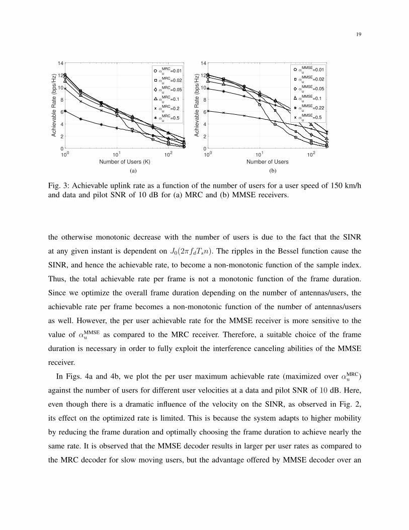
In Figs. 3a and 3b, we plot the per user achievable rates for MRC and MMSE based decoders

as a function of the number of users for different values of αMRCu . These plots assume data and

pilot SNRs of 10 dB and a user velocity of 150 km/h. The per user achievable rates drop with

an increasing number of users due to the increased interference. The increased number of users

also results in more severe aging of the available estimates which further adds to the interference

issue. The optimal value of αMRCu depends on the number of users and the pilot and data SNRs.

Its value is determined using a line search over the interval [0, 0.5]. The slight irregularities in

19

100

101

102

Number of Users (K)

0

2

4

6

8

10

12

14

Achie

vable

Rate

(bps/H

z) u

MRC=0.01

u

MRC=0.02

u

MRC=0.05

u

MRC=0.1

u

MRC=0.2

u

MRC=0.5

(a)

100

101

102

Number of Users

0

2

4

6

8

10

12

14

Achie

vable

Rate

(bps/H

z) u

MMSE=0.01

u

MMSE=0.02

u

MMSE=0.05

u

MMSE=0.1

u

MMSE=0.22

u

MMSE=0.5

(b)

Fig. 3: Achievable uplink rate as a function of the number of users for a user speed of 150 km/hand data and pilot SNR of 10 dB for (a) MRC and (b) MMSE receivers.

the otherwise monotonic decrease with the number of users is due to the fact that the SINR

at any given instant is dependent on J0(2πfdTsn). The ripples in the Bessel function cause the

SINR, and hence the achievable rate, to become a non-monotonic function of the sample index.

Thus, the total achievable rate per frame is not a monotonic function of the frame duration.

Since we optimize the overall frame duration depending on the number of antennas/users, the

achievable rate per frame becomes a non-monotonic function of the number of antennas/users

as well. However, the per user achievable rate for the MMSE receiver is more sensitive to the

value of αMMSEu as compared to the MRC receiver. Therefore, a suitable choice of the frame

duration is necessary in order to fully exploit the interference canceling abilities of the MMSE

receiver.

In Figs. 4a and 4b, we plot the per user maximum achievable rate (maximized over αMRCu )

against the number of users for different user velocities at a data and pilot SNR of 10 dB. Here,

even though there is a dramatic influence of the velocity on the SINR, as observed in Fig. 2,

its effect on the optimized rate is limited. This is because the system adapts to higher mobility

by reducing the frame duration and optimally choosing the frame duration to achieve nearly the

same rate. It is observed that the MMSE decoder results in larger per user rates as compared to

the MRC decoder for slow moving users, but the advantage offered by MMSE decoder over an

20

100

101

102

Number of Users (K)

0

2

4

6

8

10

12

14

Achie

vable

Rate

(bps/H

z)

v=10 km/h

v=50 km/h

v=100 km/h

v=150 km/h

v=200 km/h

v=250 km/h

(a)

100

101

102

Number of Users (K)

0

2

4

6

8

10

12

14

Achie

vable

Rate

(bps/H

z)

v=10 km/h

v=50 km/h

v=100 km/h

v=150 km/h

v=200 km/h

v=250 km/h

(b)

Fig. 4: Achievable uplink rate optimized over (a) αMRCu and (b) αMMSE

u as a function of thenumber of users for different user speeds, and data and pilot SNR of 10 dB.

MRC decoder (see Fig. 4a) reduces with an increase in the user mobility. This is in accordance

with the observations made from (44).

V. DOWNLINK DATA RATES

In this section, we derive the DEs of the downlink SINRs as seen by the cellular users, with

the matched filtering (MF) and the RZF precoders being used at the base stations [12], [14].

The base station transmits data symbols during the time instants N + 1 ≤ n ≤ Td. It is also

assumed the noisy and aged CSI available at the users is made available to the base station

at time (N + 1) through an ideal feedback channel. Letting sk[n] be the symbol transmitted

by the base station to the kth user at the nth time instant with an energy Ed,s,k and using a

precoder vector pk[n] ∈ CN×1, s[n] = [s1[n], s2[n], . . . , sK [n]]T , P[n] , [p1[n], . . . ,pK [n]] and

Ed,s = [Ed,s,1, . . . , Ed,s,K ]T , the symbol transmitted by the base station becomes

x[n] = P[n]diag

(√Ed,sN

)s[n]. (46)

Consequently, the signal received by the kth user at the nth instant can be expressed as

yk[n] =√βkf

(k)[n]P[n]diag

(√Ed,sN

)s[n] + wk[n]. (47)

21

Again, letting bd,k =√|ρ[N ]|2βkEd,pβkEd,p+N0

, and bd,k =√

1− b2d,k, we can describe the channel from the

kth user to the base station as the row vector f (k),

f (k)[n] = ρ[n−N ]bd,k f(k) + ρ[n−N ]bd,k f

(k) + ρ[n−N ]z(k)f [n], (48)

where f (k), f , and zf are defined respectively as the channel estimate, the channel estimation

error, and the innovation component. Substituting (48) into (47) and simplifying, we get

yk[n] = ρ[n−N ]bd,k

√βkEd,s,kN

f (k)pk[n]sk[n] +K∑m=1m 6=k

ρ[n−N ]bd,k

√βkEd,s,mN

f (k)pm[n]sm[n]

+ ρ[n−N ]bd,k

√βkEd,s,kN

f (k)pk[n]sk[n] + ρ[n−N ]

√βkEd,s,kN

z(k)f [n]pk[n]sk[n] +

√N0wk[n].

(49)

Again, the first term is the desired signal power, and all the other terms contribute to noise and

interference. In the following subsections, we use techniques similar to those in Section IV to

derive the DEs of the SINRs for different designs of the matrix P[n].

A. The MF Precoder

The matched filter precoder takes the form, P[n] = FH , such that pk[n] = f (k)H , consequently,

the received signal can be expressed as

yk[n] = ρ[n−N ]bd,k

√βkEd,s,kN

f (k)f (k)Hsk[n] +K∑m=1m 6=k

√βkEd,s,mN

f (m)f (k)Hsm[n]

+ ρ[n−N ]bd,k

√βkEd,s,kN

f (k)f (k)Hsk[n] + ρ[n−N ]

√βkEd,s,kN

z(k)k [n]f (k)Hsk[n] +

√N0wk[n].

Similar to the uplink case discussed in Section IV, the variances of the individual terms of yk[n]

can be approximated using their DEs. Therefore, the DE of the SINR at the kth user can be

computed using [12, Lemma 1], and can be expressed as

ηMFPd,k [n]−

N |ρ[n−N ]|2b2d,kβkEd,s,k

βk∑K

m=1;m 6=k Ed,s,m + |ρ[n−N ]|2b2d,kβkEd,s,k + |ρ[n−N ]|2βkEd,s,k +N0

a.s.−−→ 0.

(50)

22

Note that the pilot signals are common across users while the data signals are transmitted with

power control. In this work, we consider two types of downlink data power control, viz, equal

power allocation, and channel inversion power control. In the first scheme, the signals of all the

users are transmitted with equal powers such that Ed,s,k = Ed,s, and consequently, the downlink

SINR can be expressed as

ηMFPd,k [n]−

N |ρ[n−N ]|2b2d,kβkEd,s

(K − 1)βkEd,s + |ρ[n−N ]|2b2d,kβkEd,s + |ρ[n−N ]|2βkEd,s +N0

a.s.−−→ 0. (51)

It is to be noted that both βk and bk are decreasing functions of distance of the user from the

base station, and therefore the achievable SINR will be the minimum for a user at the cell

edge. For channel inversion based power control, each user is allocated a data power in inverse

proportionality to its long term fading coefficient βk. Hence, the SINR is given by

ηMFPd,k [n]−

N |ρ[n−N ]|2b2d,k∑K

m=1m 6=k

β−1m + |ρ[n−N ]|2b2

d,k + |ρ[n−N ]|2 + γ−1d,s

a.s.−−→ 0, (52)

with γd,s =βkEd,sN0

. In this case, the users closer to the base station will see increased interference

from the signals meant for the user located at a greater distance from the base station. Therefore,

power control for downlink massive MIMO channels in the presence of channel aging is a

nontrivial problem, and is an interesting direction for future work.

Another important observation from (50)-(52) is that with forward link training, the minimum

achievable SINR at a user is no longer a monotonically increasing function of N , the number

of base station antennas. In addition to this, a larger number of base station antennas also

increases the training duration, and reduces the effective usable time of the channel for a given

frame duration. As demonstrated in the previous section, the frame duration that maximizes

the achivable rate is a function of the number of base station antennas, the channel aging

characteristics, and the number of users. Consequently, we can optimize the minimum achievable

rate by each user by selecting a subset of the antennas from the total number of available antennas

and appropriately choosing the frame duration.

Considering equal power allocation for simplicity, we can write the achievable throughput

23

with the base station using a different codebook at each instant as

RMFPd,min = min

k

1

TMFPd

TMFPd∑

n=N+1

log2

(1 + ηMFP

d,k [TMFPd ]

). (53)

Now, since ηd,k is minimized for the farthest user, whose distance from the base station can be

approximated as the cell radius. Defining αMFPd , M

TMFPd

as the ratio of the number of antennas

used (M) to the total frame duration we can write the problem of selecting the optimal number

of base station antennas and frame duration as

maxM,αMFP

d

RMFPd,min =

M

αMFPd

αMFPdM∑

n=N+1

log2

(1 +

M |ρ[n−M ]|2b2d,min

(K − 1) + |ρ[n−M ]|2b2d,min + |ρ[n−M ]|2 + γ−1

d,min

),

(54)

where βmin = mink βk, 0 < αMFPd ≤ 1, M ≤ N , bd,min =

√|ρ[N−1]|2βminEd,pβminEd,p+N0

and γd,min =βminEd,sN0

.

Here, the optimal values of M and αMFPd can be obtained by searching over the intervals

M ∈ 1, . . . , N and αMFPd ∈ (0, 1). This is discussed in greater detail in the section on numerical

results. We next derive the DEs for SINR in case of an RZF precoder.

B. The RZF Precoder

Here, the precoding matrix can be expressed as

P[n] = Q−1

F[n]FH = (|ρ[n−K]|2FD2

dFH + d[n]IN)−1FH , (55)

with d[n] being the regularization parameter at the nth instant, and Dd = diag(√Ed,s)diag(b)diag(

√β),

and b , [b1, . . . , bK ]T . Hence,

pk[n] = Q−1

F[n]f (k)H . (56)

Using this, we can write (49) as

yk[n] = ρ[n−N ]bd,k

√βkEd,s,kN

f (k)Q−1

F[n]f (k)Hsk[n]

+K∑m=1m 6=k

bm

√βkEd,s,mN

f (m)Q−1

F[n]f (k)Hsm[n] +

K∑m=1

√βkEd,s,mN

ρ[n−N ]bd,mf (m)Q−1

F[n]f (k)Hsm[n]

+ ρ[n−N ]K∑m=1

√βkEd,s,mN

z(m)Q−1

F[n]f (k)Hsm[n] +

√N0wk[n]. (57)

24

Following steps similar to those in Appendix A, we can now show that the DE of the variance

of the desired signal can be written as

σ21,k[n]−

|ρ[n−N ]|2b2d,kβkEd,s,kNϕ2

k[n]

|1 + b2kEd,s,kβk|ρ[n−N ]|2Nϕk[n]|2

a.s.−−→ 0, (58)

where

ϕk[n] =

|ρ[n−N ]|2

N

K∑m=1m 6=k

b2mβmEd,s,m1 + em[n]

+ d[n]

−1

, (59)

and e(t)k,m[n] is computed using iterative equation below,

e(t)k,m[n] =

|ρ[n−N ]|2bmβkEd,s,m|ρ[n−K]|2

N

∑Ki=1;i 6=k

biβiEd,s,i1+e

(t−1)k,i [n]

+ d[n]

, (60)

and is initialized as e(0)k,m[n] = 1

d[n]. Similarly, the residual interference power after RZF precoding

becomes

σ22,k[n]− |ρ[n−N ]|2

βk∑

m 6=k b2mµk,m[n]Ed,s,m

|1 + b2kβkEd,s,k|ρ[n−N ]|2ϕk[n]|2

a.s.−−→ 0. (61)

where

µk,m[n] = ϕ2k,m[n] +

|b2mβkEd,s,m|2|ρ[n−N ]|4ϕ4

k,m[n]

|1 + βkEd,s,mb2m|ρ[n−N ]|2ϕk,m[n]|2

− 2<{ |b2

mβkEd,s,m||ρ[n−N ]|2ϕ3k,m

1 + |b2mβkEd,s,mρ[n−N ]|ϕk,m[n]

}), (62)

ϕk,m[n] =

(|ρ[n−N ]|2

N

K∑l=1;l 6=m,k

b2l βlEd,s,m

1 + ek,m,i[n]+ d[n]

)−1

, (63)

and ek,m,l[n] is iteratively computed as

e(t)k,m,l[n] =

|ρ[n−N ]|2N

b2l βlEd,s,l

|ρ[n−N ]|2N

∑Ki=1;i 6=m,k

b2i βiEd,s,i1+ek,m,i[n]

+ d[n]

, (64)

and is initialized as e(t)k,m,l[n] = 1

d[n]. Also, the variances of the interference components due to

25

channel estimation errors and channel aging can respectively be computed as

σ23,k[n]− |ρ[n−N ]|2 βkϕ

2k[n]

∑Km=1 b

2mEd,s,m

|1 + |ρ[n−N ]|2b2d,kβkEd,s,kϕk[n]|2

a.s.−−→ 0, (65)

and

σ24,k[n]− ρ[n−N ]|2 βkϕ

2k[n]

∑Km=1 Ed,s,m

|1 + b2d,k|ρ[n−N ]|2βkEd,s,kϕk[n]|2

a.s.−−→ 0. (66)

Considering equal downlink power being allocated to all the users, the SINR at the kth user

for N base station antennas can be expressed as

ηRZFk [N, n]

−b2d,kβkEd,sN

βkEd,s∑K

m=1m 6=k

b2d,m

µk,m[n]

ϕ2k[n]

+ βkEd,s∑K

m=1 b2m + (K − 1) |ρ[n−N ]|2

|ρ[n−N ]|2βkEd,s + N0

|ρ[n−N ]|2

a.s.−−→ 0. (67)

It can be observed that the SINR is no longer a nondecreasing function of the number of base

station antennas, therefore, similar to the MF case, we need to optimize the throughput in terms

of the number of antennas and the frame duration. Therefore, the optimization problem in terms

of the number of antennas and the frame duration can be written as

maxM,αRZF

d

RRZFd,min =

M

αRZFd

αRZFdM∑

n=N+1

log2

(1 + η1(M,n)

), (68)

subject to the constraints, βmin = mink βk, 0 < αRZFd ≤ 1, M ≤ N , bd,k =

√|ρ[N−1]|2βkEd,pβkEd,p+N0

, and

η1(M,n) = mink ηRZFk [M,n].

The optimal values of M and αRZFd can be obtained by line search. We next present numerical

results to illustrate the system tradeoff revealed by the above expressions.

C. Numerical Results

Here, we present numerical results to demonstrate the effects of channel aging on the perfor-

mance. The simulation setup is same as described in IV-C.

In Figs. 5a, and Fig 5b we plot the per user achievable rates for the MFP and the RZF

precoders as a function of the number of base station antennas, optimized over the frame duration

for different user velocities. These plot corresponds to data and pilot SNRs of 10 dB. It is

observed that at high user velocities, the use of a larger number of base station antennas results

26

101

102

103

Number of BS Antennas (N)

0

0.2

0.4

0.6

0.8

1

1.2

1.4

Achie

vable

Rate

(bps/H

z)

v=10 km/h

v=50 km/h

v=100 km/h

v=150 km/h

v=200 km/h

v=250 km/h

(a)

101

102

103

Number of BS Antennas (N)

0

0.5

1

1.5

2

2.5

3

3.5

Achie

vable

Rate

(bps/H

z) v=10 km/h

v=50 km/h

v=100 km/h

v=150 km/h

v=200 km/h

v=250 km/h

(b)

Fig. 5: Achievable downlink rate for (a) MFP and (b) RZF precoders based system as a function ofthe number of base station antennas for different user velocities for a 100 user system optimizedover the frame duration.

in a significant deterioration in the achievable rates. Consequently, the number of base station

antennas used for communication should be determined using (54). It is also observed that the

RZF precoder offers a significant advantage over the MFP for low user mobility. However, this

advantage, arising due to the cancellation of interfering streams also disappears with an increase

in user velocities. The non-monotonicity of these plots arises due to the oscillatory nature of the

Bessel function of the first order.

VI. CONCLUSIONS

In this paper, we considered the performance of an FDD massive MIMO system under channel

aging and derived the dependence of the per user achievable rate on the user mobility and the

number of base station antennas. We first derived bounds on the channel estimation error in

the presence of channel aging. Following this, we used these bounds along with DE analysis to

derive an expression for the per user achievable rate in both uplink and downlink. We considered

the MRC and the MMSE receiver in the uplink, and the MFP and the RZF precoders in the

downlink. The analysis revealed that under high user mobility, the number of base station

antennas maximizing the per user data rate for a given number of users may be less than the

number of available base station antennas. We also optimized the frame duration to maximize the

per user achivable rate. We showed that optimally choosing the frame duration and the number

27

of base station antennas is an important design issue for massive MIMO systems. Interesting

directions for future work include the optimal power allocation for uplink and downlink channels

and the study of wideband massive MIMO systems under channel aging.

APPENDIX A

DERIVATION OF σ21,k[n]

From [32], we know that

xH(A + τxxH)−1 =xHA−1

1 + τxHA−1x. (69)

Defining

Rn,k , |ρ[n−K]|2K∑m=1m6=k

b2mβmEu,s,mhmhHm + ε[n]Ik, (70)

such that Ryy|H[n] = Rn,k + |ρ[n−K]|2b2kβkEu,s,khkhHk . Therefore, we can write

|hHk R−1

yy|H[n]hk|2 =|hHk R−1

n,khk|2

|1 + |ρ[n−K]|2b2kβkEu,s,khHk R−1

n,khk|2, (71)

Also, since hk is independent of Rn,k, using [12, Lemma 1] and use (69), we get

limN→∞

1

N2|hHk R−1

n,k[n]hk|2 −1

N2|Tr(R−1

n,k)|2 a.s.−−→ 0. (72)

Now, the following result holds for a random matrix X ∈ CN×K with columns xk ∼ CN (0, 1N

Rk)

such that Rk has a uniformly bounded spectral norm with respect to M for any ρ > 0 [8],

limN→∞

1

NTr(XXH + ρIN)−1 − 1

NTr(T(ρ))

a.s.−−→ 0, (73)

where

T(ρ) =

(K∑k=1

1N

Rk

1 + ek(ρ)+ ρIN

)−1

, (74)

and ek(ρ) is iteratively computed as

e(t)k (ρ) =

1

NTr

Rk

(K∑j=1

1N

Rj

1 + e(t−1)k (ρ)

+ ρIN

)−1 , (75)

28

with the initialization e(t)k (ρ) = 1

ρ. Substituting, Rk = Nb2

kβkEu,s,k|ρ[n −K]|2IN ∀k, ρ = ε[n],

and defining ek[n] , ek(ε[n]) for simplicity we get

Tk(ρ) =

|ρ[n−K]|2K∑m=1m 6=k

βmEu,s,kb2m

1 + em[n]+ ε[n]

−1

IN . (76)

Therefore,

|hHk R−1n,k[n]hk|2 −N

|ρ[n−K]|2K∑m=1m6=k

βmEu,s,mb2m

1 + em[n]+ ε[n]

−1

a.s.−−→ 0. (77)

Defining ϕk[n] as in (35), it can be shown that

|hHk R−1

yy|H[n]hk|2 −N2ϕ2

k[n]

|1 + βkEu,s,kb2k|ρ[n−K]|Nϕk[n]|2

a.s.−−→ 0 (78)

and consequently, σ21,k[n] can be expressed as (34).

APPENDIX B

DERIVATION OF σ22,k[n]

Defining

Rn,k,m , Rn,k − b2mβmEu,s,m|ρ[n−K]|2hmhHm, (79)

and using the matrix inversion lemma [8]

(A + τxxH)−1 = A−1 − A−1τxxHA−1

1 + τxHA−1x, (80)

we can write

hHk R−1n,k[n]hm = hHk R−1

n,k,mhm − b2mβmEu,s,m|ρ[n−K]|2

×hHk R−1

n,k,mhmhHmR−1n,k,mhm

1 + βmEu,s,mb2m|ρ[n−K]|2hHmR−1

n,k,mhm. (81)

29

Consequently,

|hHk R−1n,k[n]hm|2 = |hHk R−1

n,k,mhm|2

+|b2mβmEu,s,m|2|ρ[n−K]|4|hHk R−1

n,k,mhm|2|hHmR−1n,k,mhm|2

|1 + b2mβmEu,s,m|ρ[n−K]|2hHmR−1

n,k,mhm|2

− 2<

{|b2mβmEu,s,m||ρ[n−K]|2|hHk R−1

n,k,mhm|2hHmR−1n,k,mhm

1 + βmEu,s,mb2m|ρ[n−K]|2hHmR−1

n,k,mhm

}. (82)

Since the columns of R−1n,k,m are independent w.r.t both hk and hm, we can use [12, Lemma 1]

to show that1

N|hHk R−1

n,k,mhm|2 −1

NTr(R−2

n,k,m)a.s.−−→ 0. (83)

Letting ϕk,m[n] be defined as in (39), we can write

|hHk R−1n,k,mhm|2 −Nϕ2

k,m[n]a.s.−−→ 0. (84)

Also from [12, Lemma 1],

|hHmR−1n,k,mhm|2

a.s.−−→ Tr2(R−1n,k,m)

a.s.−−→ N2ϕ2k,m[n]. (85)

Using these, σ22,k can be expressed as (37).

REFERENCES

[1] J. G. Andrews, S. Buzzi, W. Choi, S. V. Hanly, A. Lozano, A. C. K. Soong, and J. C. Zhang, “What will 5G be?” IEEE

J. Sel. Areas Commun., vol. 32, no. 6, pp. 1065–1082, Jun. 2014.

[2] K. Zheng, L. Zhao, J. Mei, B. Shao, W. Xiang, and L. Hanzo, “Survey of large-scale MIMO systems,” IEEE Commn.

Surv. Tut., vol. 17, no. 3, pp. 1738–1760, Third quarter 2015.

[3] E. G. Larsson, O. Edfors, F. Tufvesson, and T. L. Marzetta, “Massive MIMO for next generation wireless systems,” IEEE

Commun. Mag., vol. 52, no. 2, pp. 186–195, Feb. 2014.

[4] T. Narasimhan and A. Chockalingam, “Channel hardening-exploiting message passing (CHEMP) receiver in large-scale

MIMO systems,” IEEE J. Sel. Topics Signal Process., vol. 8, no. 5, pp. 847–860, Oct. 2014.

[5] L. Lu, G. Y. Li, A. L. Swindlehurst, A. Ashikhmin, and R. Zhang, “An overview of massive MIMO: Benefits and

challenges,” IEEE J. Sel. Topics Signal Process., vol. 8, no. 5, pp. 742–758, Oct. 2014.

[6] T. L. Marzetta, “Noncooperative cellular wireless with unlimited numbers of base station antennas,” IEEE Trans. Wireless

Commun., vol. 9, no. 11, pp. 3590–3600, Nov. 2010.

[7] T. L. Marzetta, E. G. Larsson, H. Yang, and H. Q. Ngo, Fundamentals of Massive MIMO. Cambridge University Press,

Cambridge, UK, 2016.

30

[8] J. Hoydis, S. ten Brink, and M. Debbah, “Massive MIMO in the UL/DL of cellular networks: How many antennas do we

need?” IEEE J. Sel. Areas Commun., vol. 31, no. 2, pp. 160–171, Feb. 2013.

[9] H. Huh, A. M. Tulino, and G. Caire, “Network MIMO with linear zero-forcing beamforming: Large system analysis, impact

of channel estimation, and reduced-complexity scheduling,” IEEE Trans. Inf. Theory, vol. 58, no. 5, pp. 2911–2934, May

2012.

[10] J. Jose, A. Ashikhmin, T. L. Marzetta, and S. Vishwanath, “Pilot contamination and precoding in multi-cell TDD systems,”

IEEE Trans. Wireless Commun., vol. 10, no. 8, pp. 2640–2651, Aug. 2011.

[11] H. Yin, D. Gesbert, M. Filippou, and Y. Liu, “A coordinated approach to channel estimation in large-scale multiple-antenna

systems,” IEEE J. Sel. Areas Commun., vol. 31, no. 2, pp. 264–273, Feb. 2013.

[12] K. T. Truong and R. W. Heath, “Effects of channel aging in massive MIMO systems,” Journal of Communications and

Networks, vol. 15, no. 4, pp. 338–351, Aug. 2013.

[13] A. K. Papazafeiropoulos, “Impact of general channel aging conditions on the downlink performance of massive MIMO,”

IEEE Trans. Veh. Technol., vol. 66, no. 2, pp. 1428–1444, Feb. 2016.

[14] A. K. Papazafeiropoulos and T. Ratnarajah, “Deterministic equivalent performance analysis of time-varying massive MIMO

systems,” IEEE Trans. Wireless Commun., vol. 14, no. 10, pp. 5795–5809, Oct. 2015.

[15] G. Amarasuriya and H. V. Poor, “Impact of channel aging in multi-way relay networks with massive MIMO,” in Proc.

IEEE Intl. Conf. Commun. (ICC 2015), London, UK, Jun. 2015, pp. 1951–1957.

[16] C. Kong, C. Zhong, A. K. Papazafeiropoulos, M. Matthaiou, and Z. Zhang, “Sum-rate and power scaling of massive MIMO

systems with channel aging,” IEEE Trans. Commun., vol. 63, no. 12, pp. 4879–4893, Dec. 2015.

[17] Q. Bao, H. Wang, Y. Chen, and C. Liu, “Downlink sum-rate and energy efficiency of massive mimo systems with channel

aging,” in Proc. 8th Int. Conf. on Wireless Commun. and Signal Process. (WCSP), Yangzhou, China, Oct. 2016, pp. 1–5.

[18] E. Bjornson, E. G. Larsson, and T. L. Marzetta, “Massive MIMO: Ten myths and one critical question,” IEEE Commun.

Mag., vol. 54, no. 2, pp. 114–123, Feb. 2016.

[19] H. Ryden, “Massive MIMO in LTE with MRT precoder: Channel aging and throughput analysis in a single-cell deployment,”

Master’s thesis, Linkoping University, Sweden, 2014.

[20] A. Papazafeiropoulos, H. Ngo, and T. Ratnarajah, “Performance of massive MIMO uplink with zero-forcing receivers

under delayed channels,” IEEE Trans. Veh. Technol., vol. 66, no. 4, pp. 3158–3169, Apr. 2017.

[21] J. Choi, D. J. Love, and P. Bidigare, “Downlink training techniques for FDD massive MIMO systems: Open-loop and

closed-loop training with memory,” IEEE J. Sel. Areas Commun., vol. 8, no. 5, pp. 802–814, Oct. 2014.

[22] A. Decurninge, M. Guillaud, and D. T. M. Slock, “Channel covariance estimation in massive MIMO frequency division

duplex systems,” in Proc. IEEE Globecom 2015 Workshops, San Diego, CA, Dec. 2015, pp. 1–6.

[23] Z. Jiang, A. F. Molisch, G. Caire, and Z. Niu, “Achievable rates of FDD massive MIMO systems with spatial channel

correlation,” IEEE Trans. Wireless Commun., vol. 14, no. 5, pp. 2868–2882, May 2015.

[24] R. Chopra, C. R. Murthy, and H. A. Suraweera, “On the throughput of large MIMO beamforming systems with channel

aging,” IEEE Signal Process. Lett., vol. 23, no. 11, pp. 1523–1527, Nov. 2016.

[25] S. Kashyap, C. Mollen, E. Bjornson, and E. G. Larsson, “Performance analysis of TDD massive MIMO with Kalman

channel predication,” in Proc. Intl. Conf. on Acoustics, Speech and Signal Processing (ICASSP 2017), New Orleans, LA,

March 2017, pp. 3554–3558.

[26] F. Rusek, D. Persson, B. K. Lau, E. G. Larsson, T. L. Marzetta, O. Edfors, and F. Tufvesson, “Scaling up MIMO:

Opportunities and challenges with very large arrays,” IEEE Signal Process. Mag., vol. 30, no. 1, pp. 40–60, Jan. 2013.

31

[27] W. C. Jakes and D. C. Cox, Eds., Microwave Mobile Communications, 2nd ed. IEEE Press, New York: IEEE Press,

1994.

[28] M. Abramowitz and I. A. Stegun, Handbook of Mathematical Functions with Formulas, Graphs, and Mathematical Tables,

9th ed. New York: Dover, 1964.

[29] B. Hassibi and B. M. Hochwald, “How much training is needed in multiple-antenna wireless links?” IEEE Trans. Inf.

Theory, vol. 49, no. 4, pp. 951–963, Apr. 2003.

[30] R. Couillet and M. Debbah, Random matrix methods for wireless communications, 1st ed. Cambridge University Press,

Cambridge, UK, 2011.

[31] A. Pitarokoilis, S. K. Mohammed, and E. G. Larsson, “Uplink performance of time-reversal mrc in massive MIMO systems

subject to phase noise,” IEEE Trans. Wireless Commun., vol. 14, pp. 711–723, Feb. 2015.

[32] J. Silverstein and Z. Bai, “On the empirical distribution of eigenvalues of a class of large dimensional

random matrices,” Journal of Multivariate Analysis, vol. 54, no. 2, pp. 175 – 192, 1995. [Online]. Available:

http://www.sciencedirect.com/science/article/pii/S0047259X85710512