Embed Size (px)
Citation preview
1 of 57Copyright © 2011 Worth Publishers· International Economics· Feenstra/Taylor, 2/e.
Cha
pter
6: I
ncre
asin
g R
etur
ns to
Sca
le a
nd M
onop
olis
tic C
ompe
titio
n
Increasing Returns to Scale and
Monopolistic Competition
Prepared by:Fernando QuijanoDickinson State University
61 Basics of Imperfect
Competition
2 Trade underMonopolisticCompetition
3 The NorthAmerican FreeTrade Agreement
4 Intra-IndustryTrade and theGravity Equation

2 of 57Copyright © 2011 Worth Publishers· International Economics· Feenstra/Taylor, 2/e.
Cha
pter
6: I
ncre
asin
g R
etur
ns to
Sca
le a
nd M
onop
olis
tic C
ompe
titio
n
Introduction
In this chapter we examine:
1. The basics of the monopolistic competition model.
2. How consumer choices and prices are affected under monopolistic competition when trade opens between two countries.
3. The gains from international trade under monopolistic competition.
4. The gains and adjustment costs for Mexico and the United States under NAFTA.
5. The gravity equation, which states that countries with higher GDP, or that are close, will trade more.

3 of 57Copyright © 2011 Worth Publishers· International Economics· Feenstra/Taylor, 2/e.
Cha
pter
6: I
ncre
asin
g R
etur
ns to
Sca
le a
nd M
onop
olis
tic C
ompe
titio
n
• Most goods are differentiated goods, that is, they are not identical.
• When we allow for imperfect competition, firms can influence the price they charge.
• Monopolistic competition has two key features:• The goods produced by different firms are
differentiated.• Firms enjoy increasing returns to scale, by which
we mean that the average costs for a firm fall as more output is produced.
Introduction

4 of 57Copyright © 2011 Worth Publishers· International Economics· Feenstra/Taylor, 2/e.
Cha
pter
6: I
ncre
asin
g R
etur
ns to
Sca
le a
nd M
onop
olis
tic C
ompe
titio
n
• Intra-industry trade deals with imports and exports in the same industry.
• Large countries (as measured by their GDP) should trade the most. This is the prediction of the gravity equation.
• The monopolistic competition model also helps us to understand the effects of free-trade agreements, in which free trade occurs among a group of countries.
• Next, we will compare and contrast the cases of monopoly and duopoly, specifically, the demand characteristics in each type of market.
Introduction

5 of 57Copyright © 2011 Worth Publishers· International Economics· Feenstra/Taylor, 2/e.
Cha
pter
6: I
ncre
asin
g R
etur
ns to
Sca
le a
nd M
onop
olis
tic C
ompe
titio
n
Monopoly Equilibrium
FIGURE 6-1
Monopoly Equilibrium
The monopolist chooses the profit-maximizing quantity, QM, at which marginal revenue equals marginal cost. From that quantity, we trace up to the demand curve and over to the price axis to see that the monopolist charges the price PM.The monopoly equilibrium is at point A.
The extra revenue earned from selling one more unit is called the marginal revenue.
1 Basics of Imperfect Competition

6 of 57Copyright © 2011 Worth Publishers· International Economics· Feenstra/Taylor, 2/e.
Cha
pter
6: I
ncre
asin
g R
etur
ns to
Sca
le a
nd M
onop
olis
tic C
ompe
titio
n
Demand with DuopolyFIGURE 6-2 (1 of 2)
Demand Curves with Duopoly
When there are two firms in the market and they both charge the same price, each firm faces the demand curve D/2.At the price P1, the industry produces Q1 at point Aand each firm produces Q2 = Q1/2 at point B.
If both firms produce identical products and one firm lowers its price to P2, all consumers will buy from that firm only;the firm that lowers its price will face the demand curve, D, and sell Q3 at point C.
1 Basics of Imperfect Competition

7 of 57Copyright © 2011 Worth Publishers· International Economics· Feenstra/Taylor, 2/e.
Cha
pter
6: I
ncre
asin
g R
etur
ns to
Sca
le a
nd M
onop
olis
tic C
ompe
titio
n
Demand with DuopolyFIGURE 6-2 (2 of 2)
Demand Curves with Duopoly
Alternatively, if the products are differentiated, the firm that lowers its price will take some, but not all, sales from the other firm; it will face the demand curve, d, and at P2 it will sell Q4 at point C′.
1 Basics of Imperfect Competition

8 of 57Copyright © 2011 Worth Publishers· International Economics· Feenstra/Taylor, 2/e.
Cha
pter
6: I
ncre
asin
g R
etur
ns to
Sca
le a
nd M
onop
olis
tic C
ompe
titio
n
Assumption 1: Each firm produces a good that is similar to but slightly differentiated from the goods that other firms in the industry produce.
• Each firm faces a downward-sloping demand curve for its product and has some control over the price it charges.
2 Trade under Monopolistic Competition
Assumptions of the model of monopolistic competition:

9 of 57Copyright © 2011 Worth Publishers· International Economics· Feenstra/Taylor, 2/e.
Cha
pter
6: I
ncre
asin
g R
etur
ns to
Sca
le a
nd M
onop
olis
tic C
ompe
titio
n
Assumption 2: There are many firms in the industry
2 Trade under Monopolistic Competition
Assumptions of the model of monopolistic competition:
• If the number of firms is N, then D/N is the share of demand that each firm faces when the firms are all charging the same price.
• When only one firm lowers its price, however, it will face a flatter demand curve d.

10 of 57Copyright © 2011 Worth Publishers· International Economics· Feenstra/Taylor, 2/e.
Cha
pter
6: I
ncre
asin
g R
etur
ns to
Sca
le a
nd M
onop
olis
tic C
ompe
titio
n
Assumption 3: Firms produce using a technology with increasing returns to scale.
FIGURE 6-3
Increasing Returns to Scale This diagram shows the average cost, AC, and marginal cost, MC, of a firm.Increasing returns to scale cause average costs to fall as the quantity produced increases. Marginal cost is below average cost and is drawn as constant for simplicity.
2 Trade under Monopolistic Competition
Assumptions of the model of monopolistic competition:
11 of 57Copyright © 2011 Worth Publishers· International Economics· Feenstra/Taylor, 2/e.
Cha
pter
6: I
ncre
asin
g R
etur
ns to
Sca
le a
nd M
onop
olis
tic C
ompe
titio
n
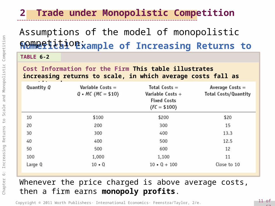
Numerical Example of Increasing Returns to ScaleTABLE 6-2
Cost Information for the Firm This table illustrates increasing returns to scale, in which average costs fall as quantity rises.
2 Trade under Monopolistic Competition
Assumptions of the model of monopolistic competition:
Whenever the price charged is above average costs, then a firm earns monopoly profits.
12 of 57Copyright © 2011 Worth Publishers· International Economics· Feenstra/Taylor, 2/e.
Cha
pter
6: I
ncre
asin
g R
etur
ns to
Sca
le a
nd M
onop
olis
tic C
ompe
titio
n
Assumption 4: Because firms can enter and exit the industry freely, monopoly profits are zero in the long run.• Firms will enter as long as it is possible to make
monopoly profits, and the more firms that enter, the lower profits per firm become.
• Profits for each firm end up as zero in the long run, just as in perfect competition.
2 Trade under Monopolistic Competition
Assumptions of the model of monopolistic competition:

13 of 57Copyright © 2011 Worth Publishers· International Economics· Feenstra/Taylor, 2/e.
Cha
pter
6: I
ncre
asin
g R
etur
ns to
Sca
le a
nd M
onop
olis
tic C
ompe
titio
n
2 Trade under Monopolistic Competition
Next, we will examine monopolistic competition:• in the short run, without trade.• in the long run, without trade.• in the short run, with free trade.• in the long run with free trade.
14 of 57Copyright © 2011 Worth Publishers· International Economics· Feenstra/Taylor, 2/e.
Cha
pter
6: I
ncre
asin
g R
etur
ns to
Sca
le a
nd M
onop
olis
tic C
ompe
titio
n
Short-Run Equilibrium
Equilibrium without Trade
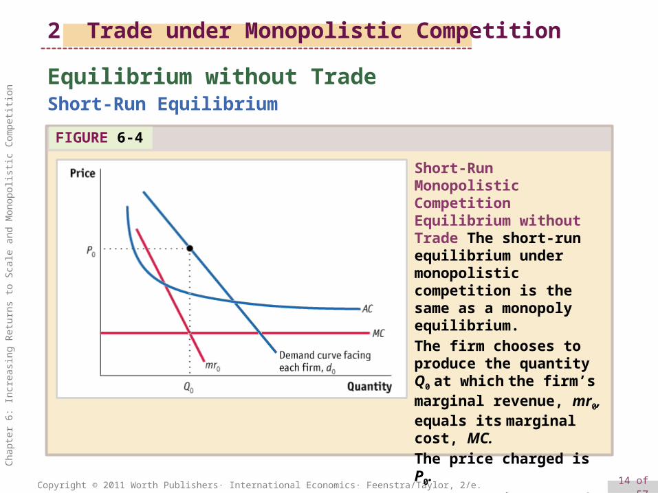
FIGURE 6-4
Short-Run Monopolistic Competition Equilibrium without Trade The short-run equilibrium under monopolistic competition is the same as a monopoly equilibrium.
The firm chooses to produce the quantity Q0 at which the firm’s marginal revenue, mr0, equals its marginal cost, MC.
The price charged is P0.
Because price exceeds average cost, the firm makes monopoly profits.
2 Trade under Monopolistic Competition

15 of 57Copyright © 2011 Worth Publishers· International Economics· Feenstra/Taylor, 2/e.
Cha
pter
6: I
ncre
asin
g R
etur
ns to
Sca
le a
nd M
onop
olis
tic C
ompe
titio
n
Long-Run EquilibriumEquilibrium without Trade
FIGURE 6-5 (1 of 2)
Long-Run Monopolistic Competition Equilibrium without Trade
Drawn by the possibility of making profits in the short-run equilibrium, new firms enter the industry and the firm’s demand curve, d0, shifts to the left and becomes more elastic (i.e., flatter), shown by d1.
The long-run equilibrium under monopolistic competition occurs at the quantity Q1 where the marginal revenue curve, mr1 (associated with demand curve d1), equals marginal cost.
At that quantity, the no-trade price, PA, equals average costs at point A.
2 Trade under Monopolistic Competition
16 of 57Copyright © 2011 Worth Publishers· International Economics· Feenstra/Taylor, 2/e.
Cha
pter
6: I
ncre
asin
g R
etur
ns to
Sca
le a
nd M
onop
olis
tic C
ompe
titio
n
Long-Run EquilibriumEquilibrium without Trade
FIGURE 6-5 (2 of 2)
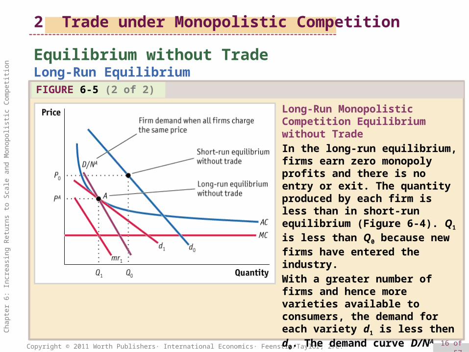
Long-Run Monopolistic Competition Equilibrium without Trade
In the long-run equilibrium, firms earn zero monopoly profits and there is no entry or exit. The quantity produced by each firm is less than in short-run equilibrium (Figure 6-4). Q1 is less than Q0 because new firms have entered the industry.
With a greater number of firms and hence more varieties available to consumers, the demand for each variety d1 is less then d0. The demand curve D/NA shows the no-trade demand when all firms charge the same price.
2 Trade under Monopolistic Competition
17 of 57Copyright © 2011 Worth Publishers· International Economics· Feenstra/Taylor, 2/e.
Cha
pter
6: I
ncre
asin
g R
etur
ns to
Sca
le a
nd M
onop
olis
tic C
ompe
titio
n
Short-Run Equilibrium with Trade
Equilibrium with Free Trade
2 Trade under Monopolistic Competition
Assume Home and Foreign are exactly the same.• Same number of consumers• Same technology and cost curves• Same number of firms in the no-trade equilibrium
Given the above conditions, if there were no economies of scale, there would be no reason for trade. Similarly,• Under the Ricardian model, countries with identical
technologies would not trade.• Under the Heckscher-Ohlin model, countries with
identical factor endowments would not trade.
However, under monopolistic competition, two identical countries will still engage in trade.

18 of 57Copyright © 2011 Worth Publishers· International Economics· Feenstra/Taylor, 2/e.
Cha
pter
6: I
ncre
asin
g R
etur
ns to
Sca
le a
nd M
onop
olis
tic C
ompe
titio
n
Short-Run Equilibrium with Trade
Equilibrium with Free Trade
2 Trade under Monopolistic Competition
• The number of firms in the no-trade equilibrium in each country is NA.
• First, we will consider each country in long-run equilibrium without trade
• When trade opens, the number of customers available to each firm doubles.
• Since there are twice as many consumers, but also twice as many firms, the ratio stays the same.
• The product varieties also double.• With the greater number of varieties available, the
demand for each individual variety will be more elastic.

19 of 57Copyright © 2011 Worth Publishers· International Economics· Feenstra/Taylor, 2/e.
Cha
pter
6: I
ncre
asin
g R
etur
ns to
Sca
le a
nd M
onop
olis
tic C
ompe
titio
n
Short-Run Equilibrium with Trade
Equilibrium with Free Trade
FIGURE 6-6 (1 of 2)
Short-Run Monopolistic Competition Equilibrium with Trade
When trade is opened, the larger market makes the firm’s demand curve more elastic, as shown by d2 (with corresponding marginal revenue curve, mr2).
The firm chooses to produce the quantity Q2 at which marginal revenue equals marginal costs;
this quantity corresponds to a price of P2. With sales of Q2 at price P2, the firm will make monopoly profits because price is greater than AC.
2 Trade under Monopolistic Competition
20 of 57Copyright © 2011 Worth Publishers· International Economics· Feenstra/Taylor, 2/e.
Cha
pter
6: I
ncre
asin
g R
etur
ns to
Sca
le a
nd M
onop
olis
tic C
ompe
titio
n
Short-Run Equilibrium with Trade
Equilibrium with Free Trade
FIGURE 6-6 (2 of 2)
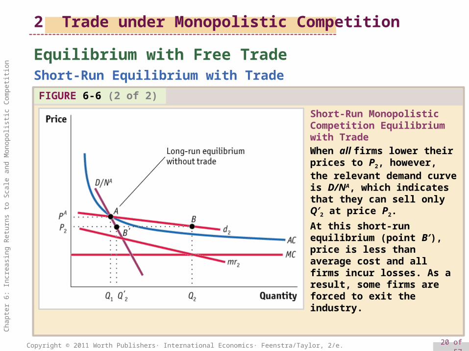
Short-Run Monopolistic Competition Equilibrium with Trade
When all firms lower their prices to P2, however, the relevant demand curve is D/NA, which indicates that they can sell only Q′2 at price P2.
At this short-run equilibrium (point B′), price is less than average cost and all firms incur losses. As a result, some firms are forced to exit the industry.
2 Trade under Monopolistic Competition

21 of 57Copyright © 2011 Worth Publishers· International Economics· Feenstra/Taylor, 2/e.
Cha
pter
6: I
ncre
asin
g R
etur
ns to
Sca
le a
nd M
onop
olis
tic C
ompe
titio
n
Long-Run Equilibrium with Trade
Equilibrium with Free Trade
2 Trade under Monopolistic Competition
• Since firms are making losses, some of them will exit the industry.
• Firm exit will increase demand for the remaining firms’ products and decrease the available product varieties to consumers.
• We now have NT firms which is fewer than the NA firms we had before.
• The new demand D/NT lies to the right of D/NA.

22 of 57Copyright © 2011 Worth Publishers· International Economics· Feenstra/Taylor, 2/e.
Cha
pter
6: I
ncre
asin
g R
etur
ns to
Sca
le a
nd M
onop
olis
tic C
ompe
titio
n
FIGURE 6-7 (1 of 2)
Long-Run Monopolistic Competition Equilibrium with Trade
The long-run equilibrium with trade occurs at point C.
At this point, profits are maximized for each firm producing Q3 (which satisfies mr3 = MC) and charging price PW (which equals AC). Since monopoly profits are zero when price equals average cost, no firms enter or exit the industry.
Long-Run Equilibrium with Trade
Equilibrium with Free Trade
2 Trade under Monopolistic Competition
23 of 57Copyright © 2011 Worth Publishers· International Economics· Feenstra/Taylor, 2/e.
Cha
pter
6: I
ncre
asin
g R
etur
ns to
Sca
le a
nd M
onop
olis
tic C
ompe
titio
n
FIGURE 6-7 (2 of 2)
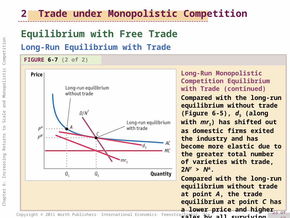
Long-Run Monopolistic Competition Equilibrium with Trade (continued)
Compared with the long-run equilibrium without trade (Figure 6-5), d3 (along with mr3) has shifted out as domestic firms exited the industry and has become more elastic due to the greater total number of varieties with trade, 2NT > NA.
Compared with the long-run equilibrium without trade at point A, the trade equilibrium at point C has a lower price and higher sales by all surviving firms.
Long-Run Equilibrium with Trade
Equilibrium with Free Trade
2 Trade under Monopolistic Competition
24 of 57Copyright © 2011 Worth Publishers· International Economics· Feenstra/Taylor, 2/e.
Cha
pter
6: I
ncre
asin
g R
etur
ns to
Sca
le a
nd M
onop
olis
tic C
ompe
titio
n
Gains from Trade
Equilibrium with Free Trade
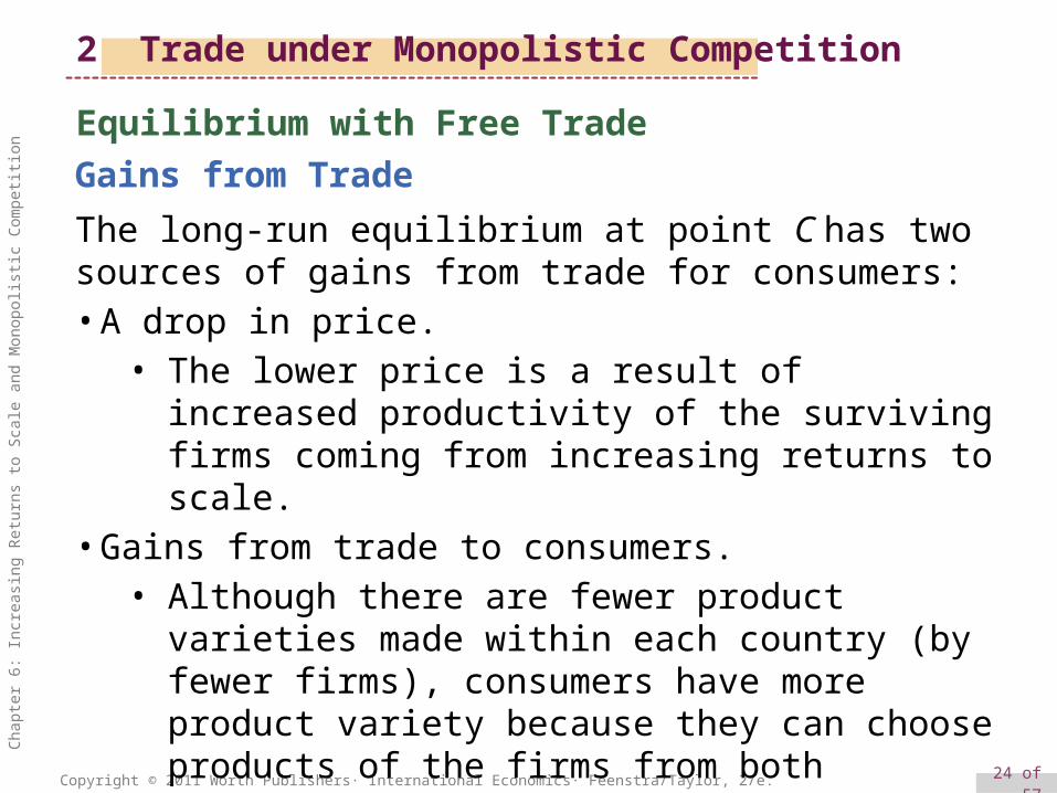
The long-run equilibrium at point C has two sources of gains from trade for consumers:• A drop in price.
• The lower price is a result of increased productivity of the surviving firms coming from increasing returns to scale.
• Gains from trade to consumers.• Although there are fewer product varieties made
within each country (by fewer firms), consumers have more product variety because they can choose products of the firms from both countries after trade.
2 Trade under Monopolistic Competition

25 of 57Copyright © 2011 Worth Publishers· International Economics· Feenstra/Taylor, 2/e.
Cha
pter
6: I
ncre
asin
g R
etur
ns to
Sca
le a
nd M
onop
olis
tic C
ompe
titio
n
Equilibrium with Free Trade
Adjustment Costs from Trade
• There are adjustment costs associated with monopolistic competition, as some firms shut down or exit the industry.
• Workers in those firms experience a spell of unemployment.
• Over the long run, however, we could expect those workers to find new jobs, so these costs are temporary.
• Feenstra shows gains and adjustment costs using NAFTA as an example.
2 Trade under Monopolistic Competition
26 of 57Copyright © 2011 Worth Publishers· International Economics· Feenstra/Taylor, 2/e.
Cha
pter
6: I
ncre
asin
g R
etur
ns to
Sca
le a
nd M
onop
olis
tic C
ompe
titio
n
Index of Intra-Industry Trade
4 Intra-Industry Trade and the Gravity Equation
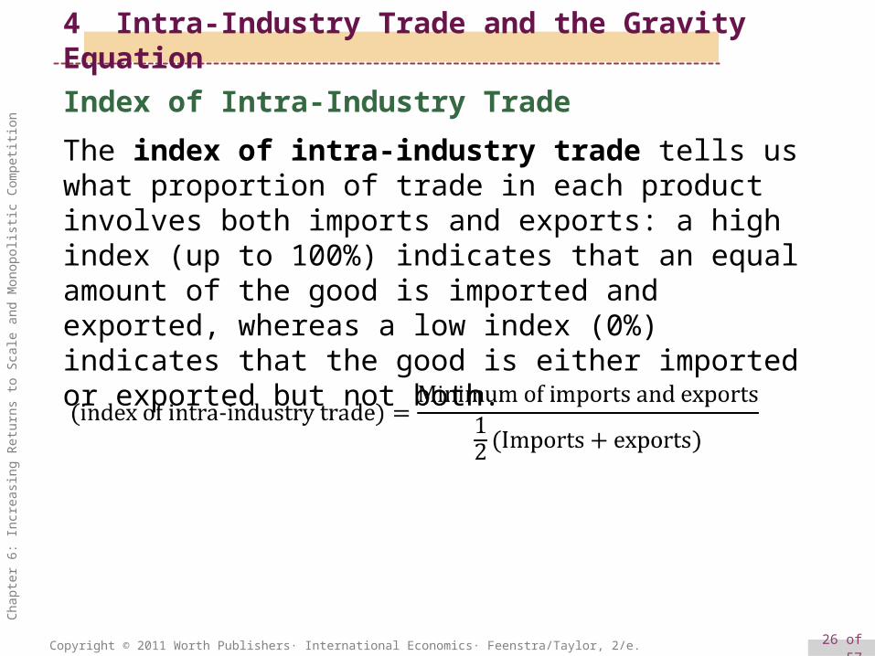
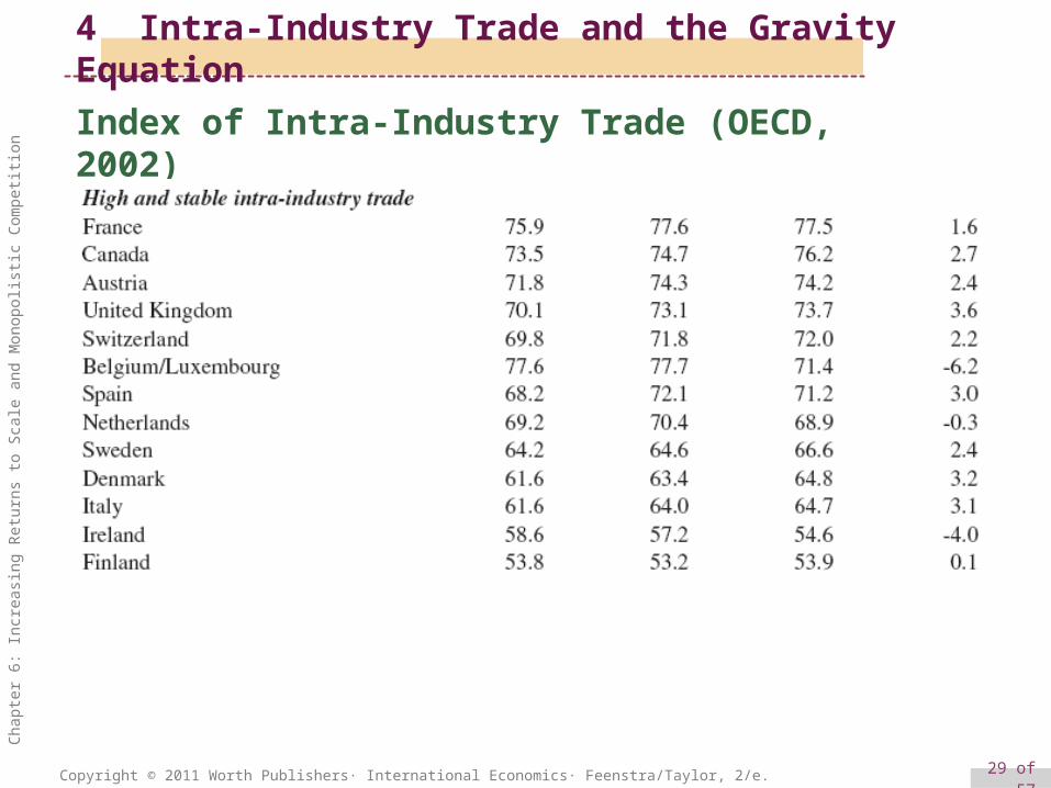
The index of intra-industry trade tells us what proportion of trade in each product involves both imports and exports: a high index (up to 100%) indicates that an equal amount of the good is imported and exported, whereas a low index (0%) indicates that the good is either imported or exported but not both.
27 of 57Copyright © 2011 Worth Publishers· International Economics· Feenstra/Taylor, 2/e.
Cha
pter
6: I
ncre
asin
g R
etur
ns to
Sca
le a
nd M
onop
olis
tic C
ompe
titio
n
Index of Intra-Industry TradeTABLE 6-4
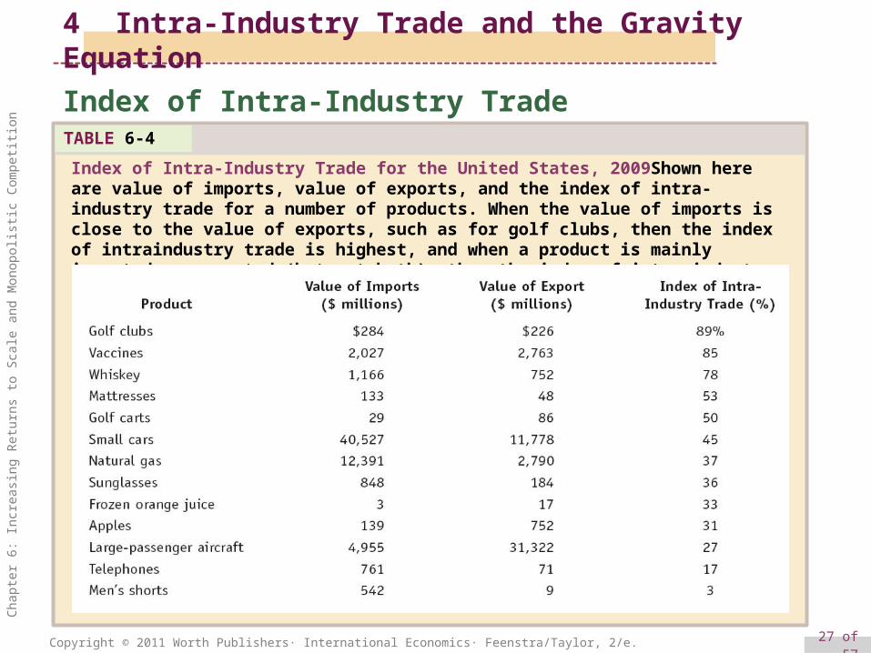
Index of Intra-Industry Trade for the United States, 2009Shown here are value of imports, value of exports, and the index of intra-industry trade for a number of products. When the value of imports is close to the value of exports, such as for golf clubs, then the index of intraindustry trade is highest, and when a product is mainly imported or exported (but not both), then the index of intra-industry trade is lowest.
4 Intra-Industry Trade and the Gravity Equation
28 of 57Copyright © 2011 Worth Publishers· International Economics· Feenstra/Taylor, 2/e.
Cha
pter
6: I
ncre
asin
g R
etur
ns to
Sca
le a
nd M
onop
olis
tic C
ompe
titio
n
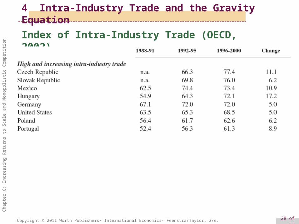
Index of Intra-Industry Trade (OECD, 2002)
4 Intra-Industry Trade and the Gravity Equation
29 of 57Copyright © 2011 Worth Publishers· International Economics· Feenstra/Taylor, 2/e.
Cha
pter
6: I
ncre
asin
g R
etur
ns to
Sca
le a
nd M
onop
olis
tic C
ompe
titio
n
Index of Intra-Industry Trade (OECD, 2002)
4 Intra-Industry Trade and the Gravity Equation

30 of 57Copyright © 2011 Worth Publishers· International Economics· Feenstra/Taylor, 2/e.
Cha
pter
6: I
ncre
asin
g R
etur
ns to
Sca
le a
nd M
onop
olis
tic C
ompe
titio
n
Index of Intra-Industry Trade (OECD, 2002)
4 Intra-Industry Trade and the Gravity Equation

31 of 57Copyright © 2011 Worth Publishers· International Economics· Feenstra/Taylor, 2/e.
Cha
pter
6: I
ncre
asin
g R
etur
ns to
Sca
le a
nd M
onop
olis
tic C
ompe
titio
n
The Gravity Equation
4 Intra-Industry Trade and the Gravity Equation
• Dutch economist and Nobel laureate, Jan Tinbergen, was trained in physics and thought of comparing the trade between countries to the force of gravity between objects.
• In physics, objects with a larger mass, or those that are close together, have greater gravitational pull between them.
• In economics, the gravity equation for trade states that countries with larger GDPs, or that are close to each other, will have more trade between them.

32 of 57Copyright © 2011 Worth Publishers· International Economics· Feenstra/Taylor, 2/e.
Cha
pter
6: I
ncre
asin
g R
etur
ns to
Sca
le a
nd M
onop
olis
tic C
ompe
titio
n
The Gravity Equation
Newton’s Universal Law of Gravitation
4 Intra-Industry Trade and the Gravity Equation
• Suppose you have two objects with masses, M1 and M2 and are located distance d apart.
• The force of gravity between these two masses is:
• The larger the objects are or the closer they are, the greater the force of gravity between them.
• In the case of trade, the larger the two countries are, or the closer they are, the greater the amount of trade.
1 22g
M MF G
d

33 of 57Copyright © 2011 Worth Publishers· International Economics· Feenstra/Taylor, 2/e.
Cha
pter
6: I
ncre
asin
g R
etur
ns to
Sca
le a
nd M
onop
olis
tic C
ompe
titio
n
The Gravity Equation
Newton’s Universal Law of Gravitation
The Gravity Equation in Trade
4 Intra-Industry Trade and the Gravity Equation
1 22g
M MF G
d
34 of 57Copyright © 2011 Worth Publishers· International Economics· Feenstra/Taylor, 2/e.
Cha
pter
6: I
ncre
asin
g R
etur
ns to
Sca
le a
nd M
onop
olis
tic C
ompe
titio
n
APPLICATION
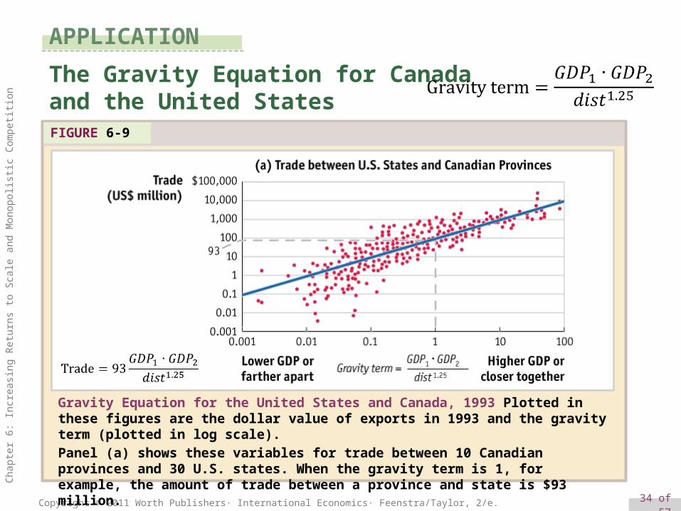
The Gravity Equation for Canadaand the United StatesFIGURE 6-9
Gravity Equation for the United States and Canada, 1993 Plotted in these figures are the dollar value of exports in 1993 and the gravity term (plotted in log scale). Panel (a) shows these variables for trade between 10 Canadian provinces and 30 U.S. states. When the gravity term is 1, for example, the amount of trade between a province and state is $93 million.
35 of 57Copyright © 2011 Worth Publishers· International Economics· Feenstra/Taylor, 2/e.
Cha
pter
6: I
ncre
asin
g R
etur
ns to
Sca
le a
nd M
onop
olis
tic C
ompe
titio
n
APPLICATION
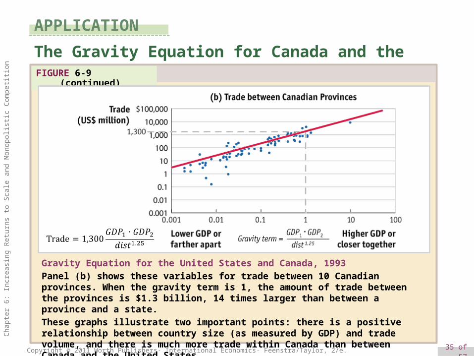
The Gravity Equation for Canada and the United StatesFIGURE 6-9 (continued)
Gravity Equation for the United States and Canada, 1993
Panel (b) shows these variables for trade between 10 Canadian provinces. When the gravity term is 1, the amount of trade between the provinces is $1.3 billion, 14 times larger than between a province and a state.
These graphs illustrate two important points: there is a positive relationship between country size (as measured by GDP) and trade volume, and there is much more trade within Canada than between Canada and the United States.

36 of 57Copyright © 2011 Worth Publishers· International Economics· Feenstra/Taylor, 2/e.
Cha
pter
6: I
ncre
asin
g R
etur
ns to
Sca
le a
nd M
onop
olis
tic C
ompe
titio
n
«New» «New» Trade theory – Marc Melitz
• Exports account for a large proportion of gross domestic product around the world, but it has come to light in recent years that only a small minority of firms actually engage in export
• The underlying idea in Melitz (2003) is that only highly productive firms are able to make sufficient profits to cover the large fixed costs required for export operations
• When lowered trade barriers stimulate competition on a global scale, low-productivity firms that had been protected by trade barriers are forced to withdraw from the market, replaced by the increased production volume of high-productivity firms. As a consequence, the average productivity of a country on the whole rises.

37 of 57Copyright © 2011 Worth Publishers· International Economics· Feenstra/Taylor, 2/e.
Cha
pter
6: I
ncre
asin
g R
etur
ns to
Sca
le a
nd M
onop
olis
tic C
ompe
titio
n
Trade theory comparison