1

Lecture 3 Innerconnection Networks for Parallel Computers

Parallel ComputingSpring 2010

2

Innerconnection Networks for Parallel Computers Interconnection networks carry data between

processors and to memory. Interconnects are made of switches and links

(wires, fiber). Interconnects are classified as static or

dynamic. Static networks

Consists of point-to-point communication links among processing nodes

Also referred to as direct networks Dynamic networks

Built using switches (switching element) and links Communication links are connected to one another

dynamically by the switches to establish paths among processing nodes and memory banks.

3

Static and DynamicInterconnection Networks

Classification of interconnection networks: (a) a static network; and (b) a dynamic network.

4

Network Topologies Bus-Based Networks

The simplest network that consists a shared medium(bus) that is common to all the nodes.

The distance between any two nodes in the network is constant (O(1)).

Ideal for broadcasting information among nodes. Scalable in terms of cost, but not scalable in terms of

performance. The bounded bandwidth of a bus places limitations on the

overall performance as the number of nodes increases. Typical bus-based machines are limited to dozens of nodes.

Sun Enterprise servers and Intel Pentium based shared-bus multiprocessors are examples of such architectures

5

Network Topologies Crossbar Networks

Employs a grid of switches or switching nodes to connect p processors to b memory banks.

Nonblocking network: the connection of a processing node to a memory bank

doesnot block the connection of any other processing nodes to other memory banks.

The total number of switching nodes required is Θ(pb). (It is reasonable to assume b>=p)

Scalable in terms of performance Not scalable in terms of cost. Examples of machines that employ crossbars include

the Sun Ultra HPC 10000 and the Fujitsu VPP500

6

Network Topologies: Multistage Network

Multistage Networks Intermediate class of networks between bus-based network and crossbar

network Blocking networks: access to a memory bank by a processor may

disallow access to another memory bank by another processor. More scalable than the bus-based network in terms of performance,

more scalable than crossbar network in terms of cost.

The schematic of a typical multistage interconnection network.

7

Network Topologies: Multistage Omega Network Omega network

Consists of log p stages, p is the number of inputs(processing nodes) and also the number of outputs(memory banks)

Each stage consists of an interconnection pattern that connects p inputs and p outputs:

Perfect shuffle(left rotation):

Each switch has two conncetion modes: Pass-thought conncetion: the inputs are sent straight

through to the outputs Cross-over connection: the inputs to the switching node

are crossed over and then sent out. Has p/2*log p switching nodes

2 , 0 / 2 1

2 1 , / 2 1

i i pj

i p p i p

8

Network Topologies: Multistage Omega Network

A complete omega network connecting eight inputs and eight outputs.

An omega network has p/2 × log p switching nodes, and the cost of such a network grows as (p log p).

A complete Omega network with the perfect shuffle interconnects and switches can now be illustrated:

9

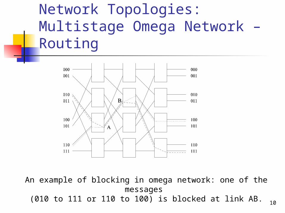
Network Topologies: Multistage Omega Network – Routing

Let s be the binary representation of the source and d be that of the destination processor.

The data traverses the link to the first switching node. If the most significant bits of s and d are the same, then the data is routed in pass-through mode by the switch else, it switches to crossover.

This process is repeated for each of the log p switching stages.

Note that this is not a non-blocking switch.

10

Network Topologies: Multistage Omega Network – Routing

An example of blocking in omega network: one of the messages (010 to 111 or 110 to 100) is blocked at link AB.

11

Network Topologies - Fixed Connection Networks (static) Completely-connection Network Star-Connected Network Linear array 2d-array or 2d-mesh or mesh 3d-mesh Complete Binary Tree (CBT) 2d-Mesh of Trees Hypercube Butterfly

12

Evaluating Static Interconnection Network

One can view an interconnection network as a graph whose nodes correspond to processors and its edges to links connecting neighboring processors. The properties of these interconnection networks can be described in terms of a number of criteria.

(1) Set of processor nodes V . The cardinality of V is the number of processors p (also denoted by n).

(2) Set of edges E linking the processors. An edge e = (u, v) is represented by a pair (u, v) of nodes. If the graph G = (V,E) is directed, this means that there is a unidirectional link from processor u to v. If the graph is undirected, the link is bidirectional. In almost all networks that will be considered in this course communication links will be bidirectional. The exceptions will be clearly distinguished.

(3) The degree du of node u is the number of links containing u as an endpoint. If graph G is directed we distinguish between the out-degree of u (number of pairs (u, v) ∈ E, for any v ∈ V ) and similarly, the in-degree of u. T he degree d of graph G is the maximum of the degrees of its nodes i.e. d = maxudu.

13

Evaluating Static Interconnection Network (cont.) (4) The diameter D of graph G is the maximum of the lengths of

the shortest paths linking any two nodes of G. A shortest path between u and v is the path of minimal length linking u and v. We denote the length of this shortest path by duv. Then, D = maxu,vduv. The diameter of a graph G denotes the maximum delay (in terms of number of links traversed) that will be incurred when a packet is transmitted from one node to the other of the pair that contributes to D (i.e. from u to v or the other way around, if D = duv). Of course such a delay would hold if messages follow shortest paths (the case for most routing algorithms).

(5) latency is the total time to send a message including software overhead. Message latency is the time to send a zero-length message.

(6) bandwidth is the number of bits transmitted in unit time. (7) bisection width is the number of links that need to be

removed from G to split the nodes into two sets of about the same size (±1).

14

Network Topologies - Fixed Connection Networks (static) Completely-connection Network

Each node has a direct communication link to every other node in the network.

Ideal in the sense that a node can send a message to another node in a single step.

Static counterpart of crossbar switching networks Nonblocking

Star-Connected Network One processor acts as the central processor. Every

other processor has a communication link connecting it to this central processor.

Similar to bus-based network. The central processor is the bottleneck.

15

Network Topologies: Completely Connected and Star Connected Networks

Example of an 8-node completely connected network.

(a) A completely-connected network of eight nodes; (b) a star connected network of nine nodes.

16

Network Topologies - Fixed Connection Networks (static) Linear array

In a linear array, each node(except the two nodes at the ends) has two neighbors, one each to its left and right.

Extension: ring or 1-D torus(linear array with wraparound). 2d-array or 2d-mesh or mesh

The processors are ordered to form a 2-dimensional structure (square) so that each processor is connected to its four neighbor (north, south, east, west) except perhaps for the processors of the boundary.

Extension of linear array to two-dimensions: Each dimension has p nodes with a node identified by a two-tuple (i,j).

3d-mesh A generalization of a 2d-mesh in three dimensions. Exercise: Find the

characteristics of this network and its generalization in k dimensions (k > 2).

Complete Binary Tree (CBT) There is only one path between any pair of two nodes Static tree network: have a processing element at each node of the tree. Dynamic tree network: nodes at intermediate levels are switching nodes

and the leaf nodes are processing elements. Communication bottleneck at higher levels of the tree.

Solution: increasing the number of communication links and switching nodes closer to the root.

17

Network Topologies: Linear Arrays

Linear arrays: (a) with no wraparound links; (b) with wraparound link.

18

Network Topologies: Two- and Three Dimensional Meshes

Two and three dimensional meshes: (a) 2-D mesh with no wraparound; (b) 2-D mesh with wraparound link (2-D torus); and

(c) a 3-D mesh with no wraparound.

19

Network Topologies: Tree-Based Networks

Complete binary tree networks: (a) a static tree network; and (b) a dynamic tree network.

20

Network Topologies: Fat Trees

A fat tree network of 16 processing nodes.

21

Evaluating Network Topologies Linear array

|V | = N, |E| = N −1, d = 2, D = N −1, bw = 1 (bisection width).

2d-array or 2d-mesh or mesh For |V | = N, we have a √N ×√N mesh structure, with |E| ≤

2N = O(N), d = 4, D = 2√N − 2, bw = √N. 3d-mesh

Exercise: Find the characteristics of this network and its generalization in k dimensions (k > 2).

Complete Binary Tree (CBT) on N = 2n leaves For a complete binary tree on N leaves, we define the level

of a node to be its distance from the root. The root is of level 0 and the number of nodes of level i is 2i. Then, |V | = 2N − 1, |E| ≤ 2N − 2 = O(N), d = 3, D = 2lgN, bw = 1(c)

22

Network Topologies - Fixed Connection Networks (static) 2d-Mesh of Trees

An N2-leaf 2d-MOT consists of N2 nodes ordered as in a 2d-array N ×N (but without the links). The N rows and N columns of the 2d-MOT form N row CBT and N column CBTs respectively.

For such a network, |V | = N2+2N(N −1), |E| = O(N2), d = 3, D = 4lgN, bw = N. The 2d-MOT possesses an interesting decomposition property. If the 2N roots of the CBT’s are removed we get 4 N/2 × N/2 CBT s.

The 2d-Mesh of Trees (2d-MOT) combines the advantages of 2d-meshes and binary trees. A 2d-mesh has large bisection width but large diameter (√N). On the other hand a binary tree on N leaves has small bisection width but small diameter. The 2d-MOT has small diameter and large bisection width.

A 3d-MOTcan be defined similarly.

23

Network Topologies - Fixed Connection Networks (static)

Hypercube The hypercube is the major representative of a class of networks that are

called hypercubic networks. Other such networks is the butterfly, the shuffle-exchange graph, de-Bruijn graph, Cube-connected cycles etc.

Each vertex of an n-dimensional hypercube is represented by a binary string of length n. Therefore there are |V | = 2n = N vertices in such a hypercube. Two vertices are connected by an edge if their strings differ in exactly one bit position.

Let u = u1u2 . . .ui . . . un. An edge is a dimension i edge if it links two nodes that differ in the i-th bit position.

This way vertex u is connected to vertex ui= u1u2 . . . ūi . . .un with a dimension i edge. Therefore |E| = N lg N/2 and d = lgN = n.

The hypercube is the first network examined so far that has degree that is not a constant but a very slowly growing function of N. The diameter of the hypercube is D = lgN. A path from node u to node v can be determined by correcting the bits of u to agree with those of v starting from dimension 1 in a “left-to-right” fashion. The bisection width of the hypercube is bw = N. This is a result of the following property of the hypercube. If all edges of dimension i are removed from an n dimensional hypercube, we get two hypercubes each one of dimension n − 1.

24

Network Topologies: Hypercubes and their Construction

Construction of hypercubes from hypercubes of lower dimension.

25

Network Topologies - Fixed Connection Networks (static) Butterfly.

The set of vertices of a butterfly are represented by (w, i), where w is a binary string of length n and 0 ≤ i ≤ n.

Therefore |V | = (n + 1)2n = (lgN + 1)N. Two vertices (w, i) and (w’, i’ ) are connected by an edge if i‘ = i + 1 and either (a) w = w’ or (b) w and w’ differ in the i’ bit. As a result |E| = O(N lgN), d = 4, D = 2lgN = 2n, and bw = N.

Nodes with i = j are called level-j nodes. If we remove the nodes of level 0 we get two butterflies of size N/2. If we collapse all levels of an n dimensional butterfly into one, we get a hypercube.

26

Network Topologies - Fixed Connection Networks (static) Other:

Other hypercubic networks is cube-connected cycles (CCC), which is a hypercube whose nodes are replaced by rings/cycles of length n so that the resulting network has constant degree). This network can also be viewed as a butterfly whose first and last levels collapse into one. For such a network |V | = N lgN = n2n, |E| = 3n2n−1, d = 3, D = 2lgN, bw = N/2.

27

Evaluating Static Interconnection Networks

Network Diameter BisectionWidth

Arc Connectivity

Cost (No. of links)

Completely-connected

Star

Complete binary tree

Linear array

2-D mesh, no wraparound

2-D wraparound mesh

Hypercube

Wraparound k-ary d-cube

28

End

Thank you!