Embed Size (px)
Citation preview
1
Game MathematicsGame Mathematics
2
MatricesMatrices VectorsVectors Fixed-point Real NumbersFixed-point Real Numbers Triangle MathematicsTriangle Mathematics Intersection IssuesIntersection Issues Euler AnglesEuler Angles Angular DisplacementAngular Displacement QuaternionQuaternion Differential Equation BasicsDifferential Equation Basics
Essential Mathematics for Game DevelopmentEssential Mathematics for Game Development
3
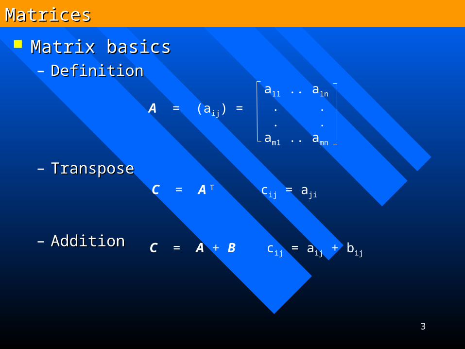
Matrix basicsMatrix basics– DefinitionDefinition
– TransposeTranspose
– AdditionAddition
MatricesMatrices
A = (aij) =
a11 .. a1n
. . . .am1 .. amn
C = A T cij = aji
C = A + B cij = aij + bij
4
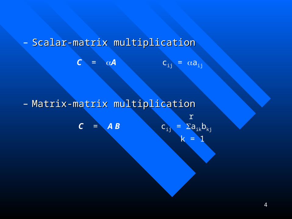
– Scalar-matrix multiplicationScalar-matrix multiplication
– Matrix-matrix multiplicationMatrix-matrix multiplication
C = A cij = aij
C = A B cij = aikbkj
k = 1
r
5
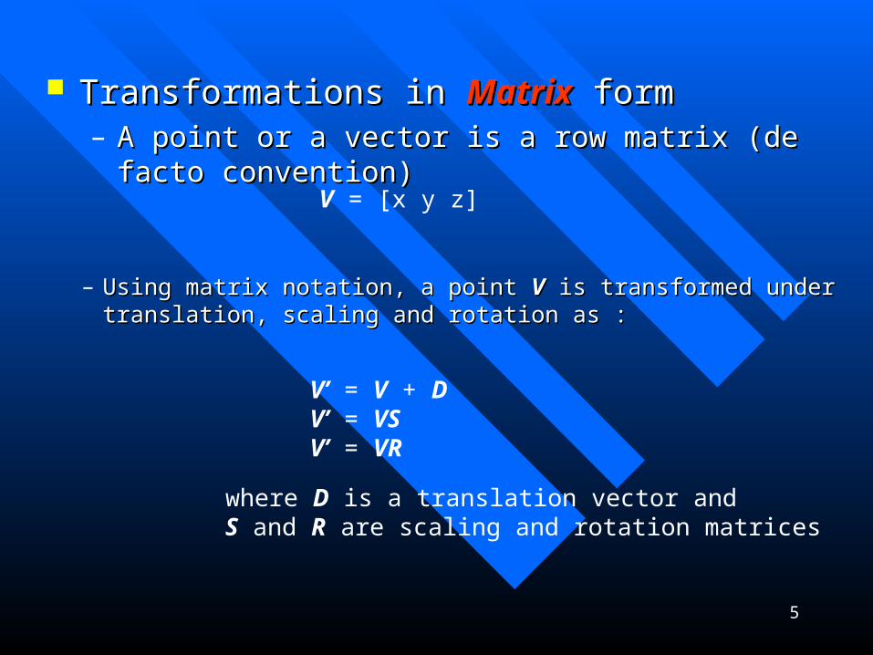
Transformations in Transformations in MatrixMatrix form form– A point or a vector is a row matrix (de facto convention)A point or a vector is a row matrix (de facto convention)
V = [x y z]
– Using matrix notation, a point Using matrix notation, a point VV is transformed under translation, is transformed under translation, scaling and rotation as :scaling and rotation as :
V’ = V + DV’ = VSV’ = VR
where D is a translation vector andS and R are scaling and rotation matrices
6
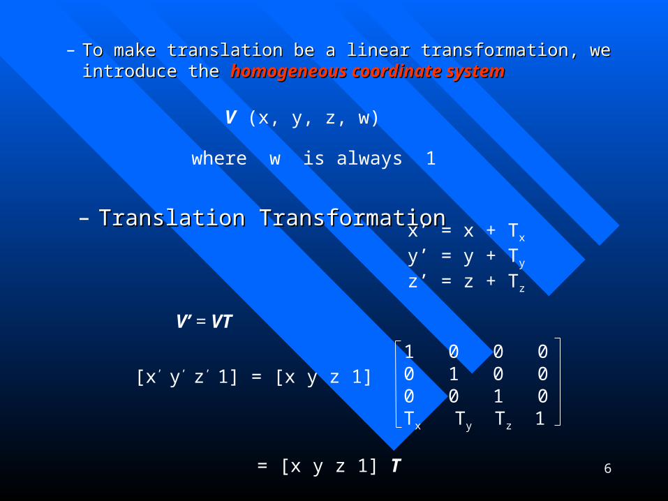
– To make translation be a linear transformation, we introduce the To make translation be a linear transformation, we introduce the homogeneous coordinate systemhomogeneous coordinate system
V (x, y, z, w)
where w is always 1
– Translation TransformationTranslation Transformationx’ = x + Tx
y’ = y + Ty
z’ = z + Tz
V’ = VT
[x’ y’ z’ 1] = [x y z 1]
= [x y z 1] T
1 0 0 00 1 0 00 0 1 0Tx Ty Tz 1
7
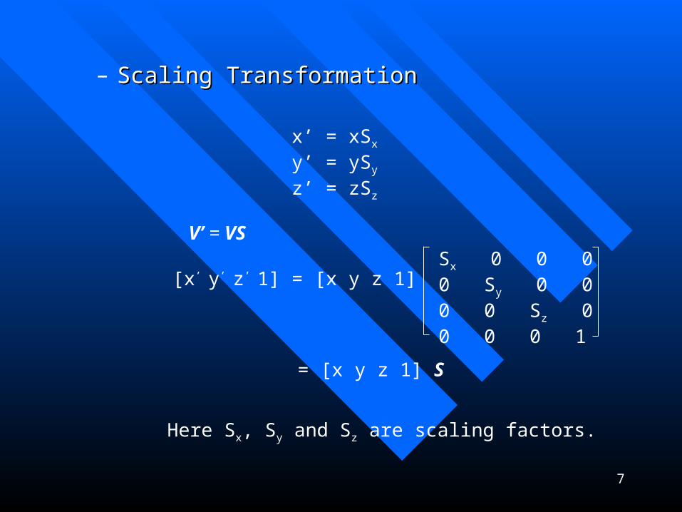
– Scaling TransformationScaling Transformation
x’ = xSx
y’ = ySy
z’ = zSz
V’ = VS
[x’ y’ z’ 1] = [x y z 1]
= [x y z 1] S
Sx 0 0 00 Sy 0 00 0 Sz 00 0 0 1
Here Sx, Sy and Sz are scaling factors.
8
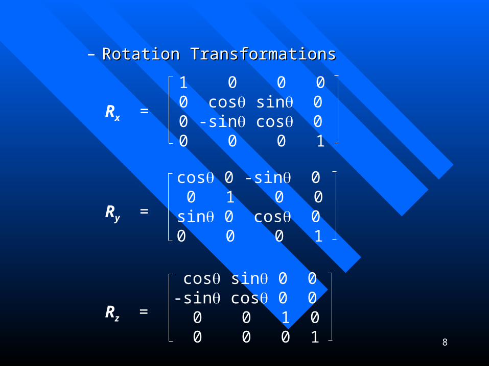
– Rotation TransformationsRotation Transformations
1 0 0 00 cos sin 00 -sin cos 00 0 0 1
Rx =
Ry =
Rz =
cos 0 -sin 0 0 1 0 0sin 0 cos 00 0 0 1
cos sin 0 0-sin cos 0 0 0 0 1 0 0 0 0 1
9
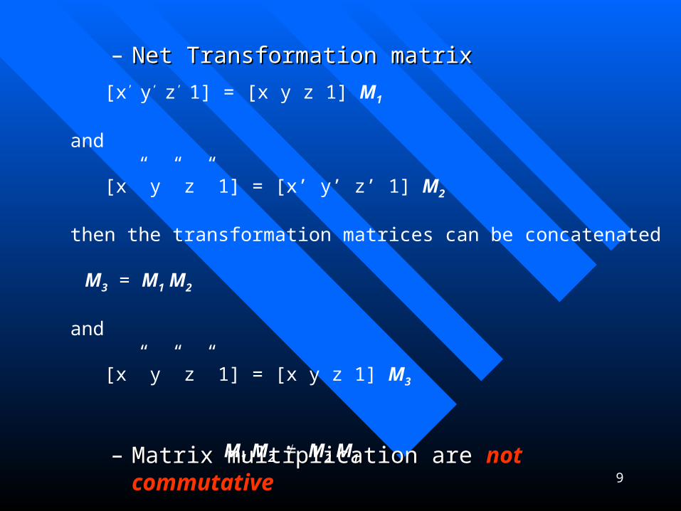
– Net Transformation matrixNet Transformation matrix
– Matrix multiplication are Matrix multiplication are not commutativenot commutative
[x’ y’ z’ 1] = [x y z 1] M1
and
[x” y” z” 1] = [x’ y’ z’ 1] M2
then the transformation matrices can be concatenated
M3 = M1 M2
and
[x” y” z” 1] = [x y z 1] M3
M1 M2 = M2 M1
10
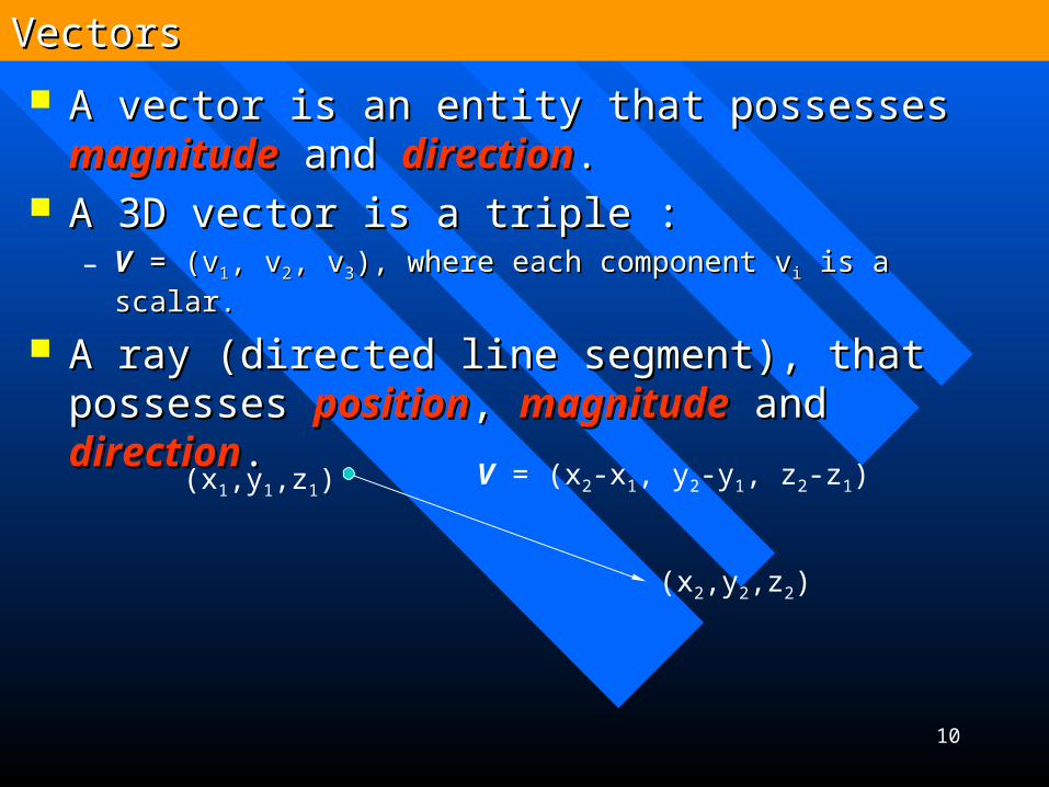
A vector is an entity that possesses A vector is an entity that possesses magnitudemagnitude an and d directiondirection..
A 3D vector is a triple :A 3D vector is a triple :– VV = (v = (v11, v, v22, v, v33)), where each component , where each component vvii is a scalar. is a scalar.
A ray (directed line segment), that possesses A ray (directed line segment), that possesses positionposition, , magnitudemagnitude and and directiondirection..
VectorsVectors
(x1,y1,z1)
(x2,y2,z2)
V = (x2-x1, y2-y1, z2-z1)
11
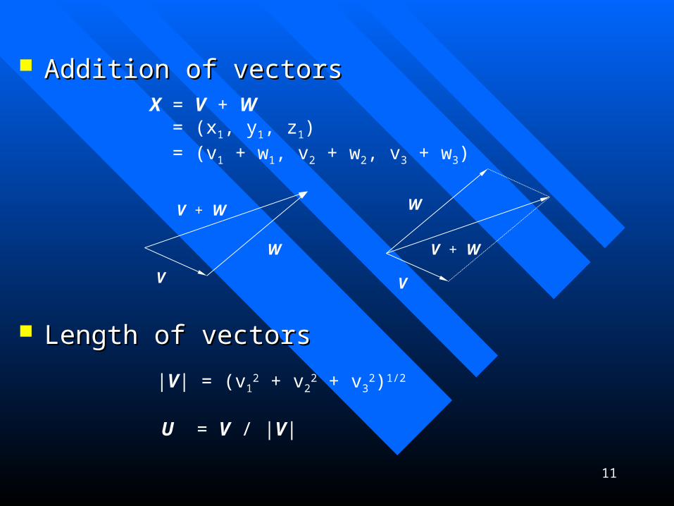
AddAddiition of vectorstion of vectors
Length of vectorsLength of vectors
X = V + W = (x1, y1, z1) = (v1 + w1, v2 + w2, v3 + w3)
V
W
V + W
V
W
V + W
|V| = (v12 + v2
2 + v32)1/2
U = V / |V|
12
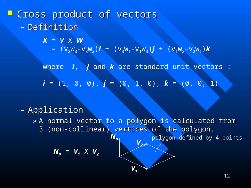
Cross product of vectorsCross product of vectors– DefinitionDefinition
– ApplicationApplication» A normal vector to a polygon is calculated from 3 (non-collinear) A normal vector to a polygon is calculated from 3 (non-collinear)
vertices of the polygon.vertices of the polygon.
X = V X W = (v2w3-v3w2)i + (v3w1-v1w3)j + (v1w2-v2w1)k
where i, j and k are standard unit vectors :
i = (1, 0, 0), j = (0, 1, 0), k = (0, 0, 1)
NpV2
V1
polygon defined by 4 points
Np = V1 X V2
13
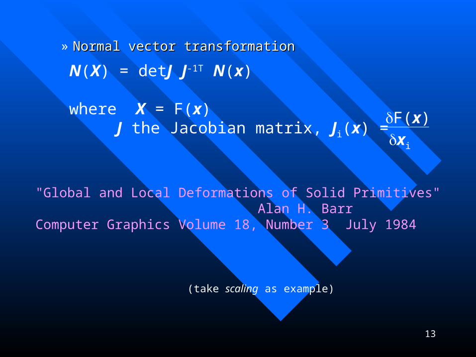
» Normal vector transformationNormal vector transformation
N(X) = detJ J-1T N(x)
where X = F(x) J the Jacobian matrix, Ji(x) =
F(x)xi
(take scaling as example)
"Global and Local Deformations of Solid Primitives" Alan H. BarrComputer Graphics Volume 18, Number 3 July 1984
14
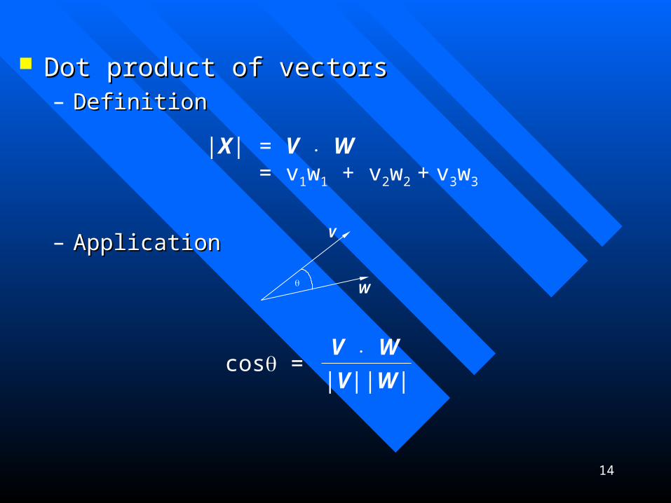
Dot product of vectorsDot product of vectors– DefinitionDefinition
– ApplicationApplication
|X| = V . W = v1w1 + v2w2 + v3w3
V
W
cos =V . W
|V||W|
15
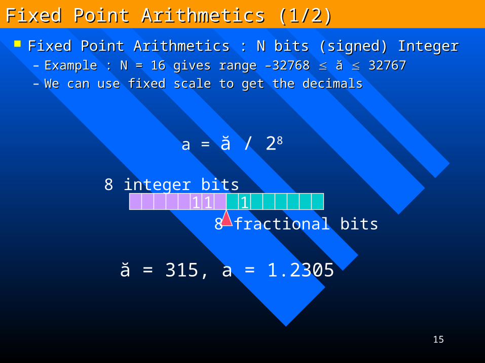
Fixed Point Arithmetics : N bits (signed) IntegerFixed Point Arithmetics : N bits (signed) Integer– Example : N = 16 gives range –32768 Example : N = 16 gives range –32768 ă ă 32767 32767– We can use fixed scale to get the decimalsWe can use fixed scale to get the decimals
Fixed Point Arithmetics (1/2)Fixed Point Arithmetics (1/2)
a = ă / 28
1 1 18 integer bits
8 fractional bits
ă = 315, a = 1.2305
16
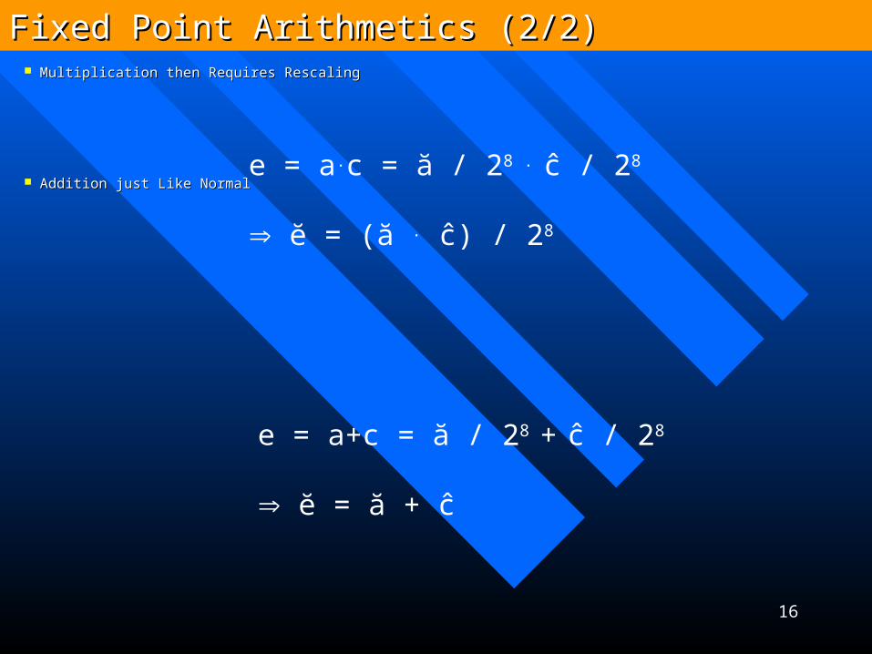
Multiplication then Requires RescalingMultiplication then Requires Rescaling
Addition just Like Normal Addition just Like Normal
Fixed Point Arithmetics (2/2)Fixed Point Arithmetics (2/2)
e = a.c = ă / 28 . ĉ / 28
ĕ = (ă . ĉ) / 28
e = a+c = ă / 28 + ĉ / 28
ĕ = ă + ĉ
17
Compression for Floating-point Real Compression for Floating-point Real NumbersNumbers– 4 bits reduced to 2 bits4 bits reduced to 2 bits– Lost some accuracy but affordableLost some accuracy but affordable– Network data transferNetwork data transfer
Software 3D RenderingSoftware 3D Rendering
Fixed Point Arithmetics - ApplicationFixed Point Arithmetics - Application
18
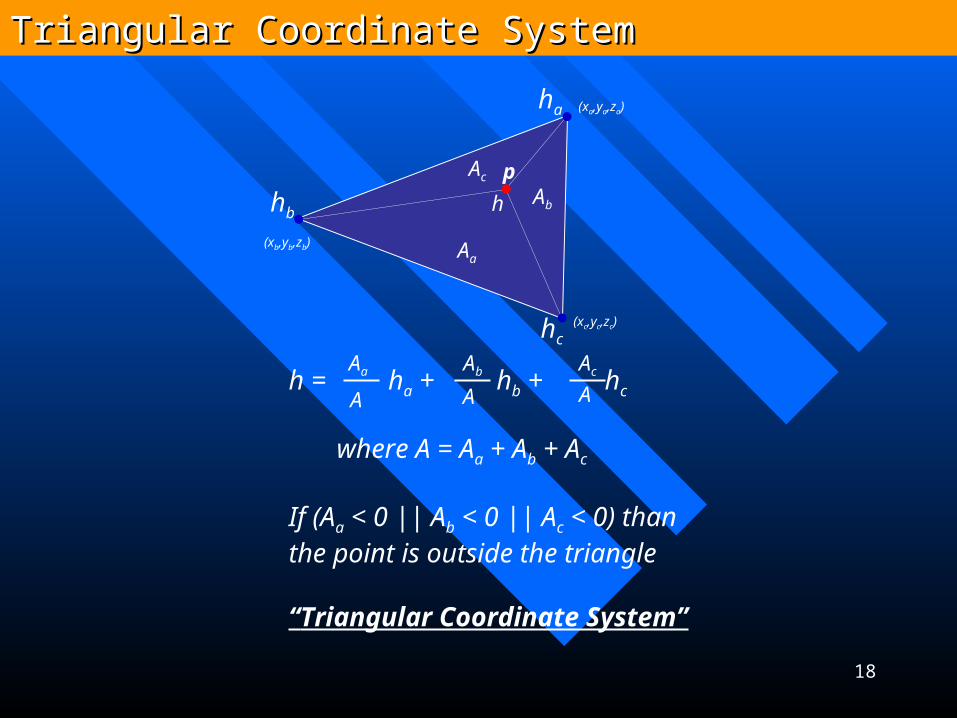
h
ha
hb
hc
Aa
Ac
Ab
h = ha + hb + hc
where A = Aa + Ab + Ac
If (Aa < 0 || Ab < 0 || Ac < 0) thanthe point is outside the triangle
“Triangular Coordinate System”
Aa Ab Ac
A A A
p
(xa,ya,za)
(xb,yb,zb)
(xc,yc,zc)
Triangular Coordinate SystemTriangular Coordinate System
19
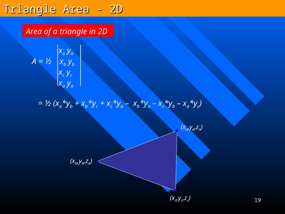
Area of a triangle in 2D
xa ya
A = ½ xb yb
xc yc
xa ya
= ½ (xa*yb + xb*yc + xc*ya – xb*ya – xc*yb – xa*yc)
Triangle Area – 2DTriangle Area – 2D
(xa,ya,za)
(xb,yb,zb)
(xc,yc,zc)
20
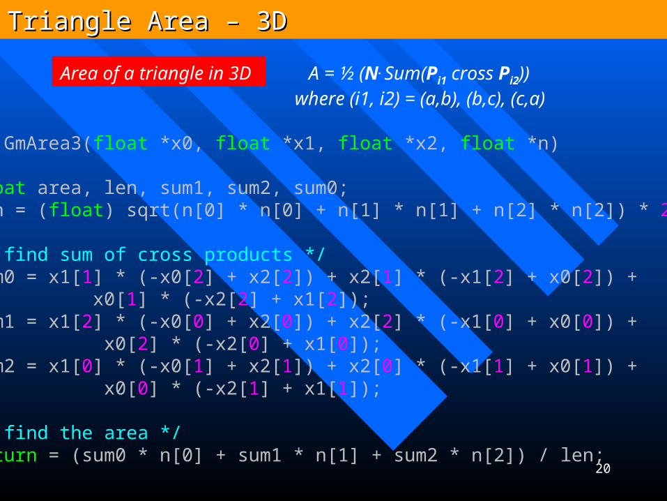
Area of a triangle in 3D A = ½ (N. Sum(Pi1 cross Pi2)) where (i1, i2) = (a,b), (b,c), (c,a)
Triangle Area – 3DTriangle Area – 3D
float GmArea3(float *x0, float *x1, float *x2, float *n){ float area, len, sum1, sum2, sum0; len = (float) sqrt(n[0] * n[0] + n[1] * n[1] + n[2] * n[2]) * 2.0f;
/* find sum of cross products */ sum0 = x1[1] * (-x0[2] + x2[2]) + x2[1] * (-x1[2] + x0[2]) + x0[1] * (-x2[2] + x1[2]); sum1 = x1[2] * (-x0[0] + x2[0]) + x2[2] * (-x1[0] + x0[0]) + x0[2] * (-x2[0] + x1[0]); sum2 = x1[0] * (-x0[1] + x2[1]) + x2[0] * (-x1[1] + x0[1]) + x0[0] * (-x2[1] + x1[1]);
/* find the area */ return = (sum0 * n[0] + sum1 * n[1] + sum2 * n[2]) / len;}
21
Terrain FollowingTerrain Following Hit TestHit Test Ray CastRay Cast Collision DetectionCollision Detection
Triangular Coordinate System - ApplicationTriangular Coordinate System - Application
22
Ray CastRay Cast Containment TestContainment Test
IntersectionIntersection
23
Ray Cast – The RayRay Cast – The Ray
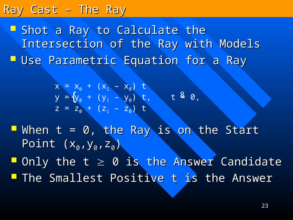
x = x0 + (x1 – x0) ty = y0 + (y1 – y0) t, t = 0,z = z0 + (z1 – z0) t
{
Shot a Ray to Calculate the Intersection of the Shot a Ray to Calculate the Intersection of the Ray with ModelsRay with Models
Use Parametric Equation for a RayUse Parametric Equation for a Ray
8
When t = 0, the Ray is on the Start Point When t = 0, the Ray is on the Start Point (x(x00,y,y00,z,z00))
Only the t Only the t 0 is the Answer Candidate 0 is the Answer Candidate The Smallest Positive t is the AnswerThe Smallest Positive t is the Answer
24
Ray Cast – The PlaneRay Cast – The Plane
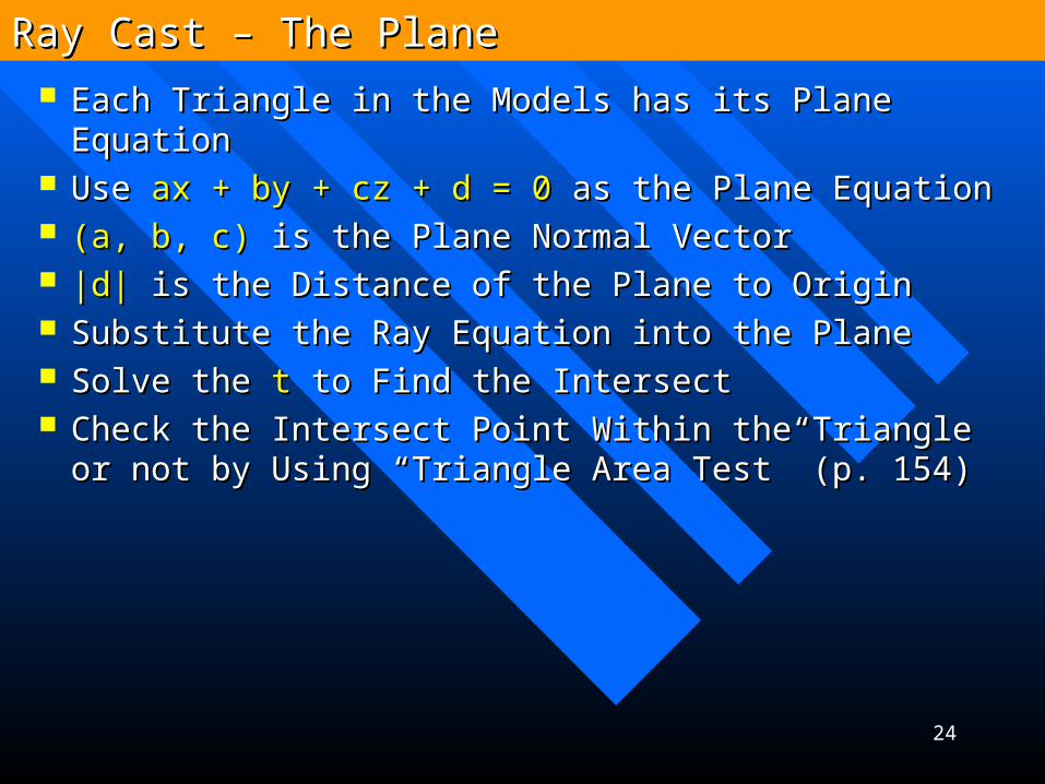
Each Triangle in the Models has its Plane Each Triangle in the Models has its Plane EquationEquation
UUse se ax + by + cz + d = 0ax + by + cz + d = 0 as the Plane Equation as the Plane Equation ((a, b, c)a, b, c) is the Plane Normal Vector is the Plane Normal Vector |d||d| is the Distance of the Plane to Origin is the Distance of the Plane to Origin Substitute the Ray Equation into the PlaneSubstitute the Ray Equation into the Plane SSolve the olve the tt to Find the Intersect to Find the Intersect CCheck the Intersect Point Within the Triangle or heck the Intersect Point Within the Triangle or
not by Using “Triangle Area Test” (p. 154)not by Using “Triangle Area Test” (p. 154)
25
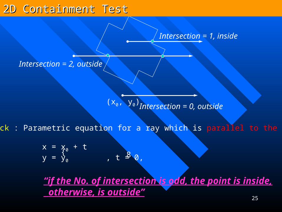
Intersection = 1, inside
Intersection = 2, outside
Intersection = 0, outside
Trick : Parametric equation for a ray which is parallel to the x-axis
x = x0 + t y = y0 , t = 0,
{ 8
(x0, y0)
2D Containment Test2D Containment Test
“ if the No. of intersection is odd, the point is inside, otherwise, is outside”
26
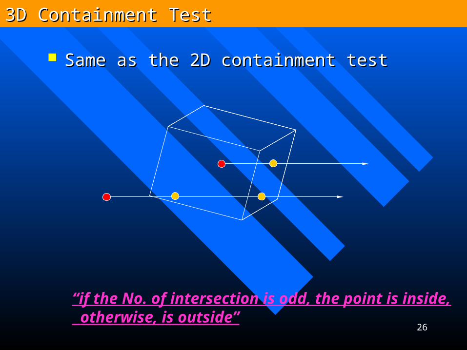
3D Containment Test3D Containment Test
“ if the No. of intersection is odd, the point is inside, otherwise, is outside”
Same as the 2D containment testSame as the 2D containment test
27
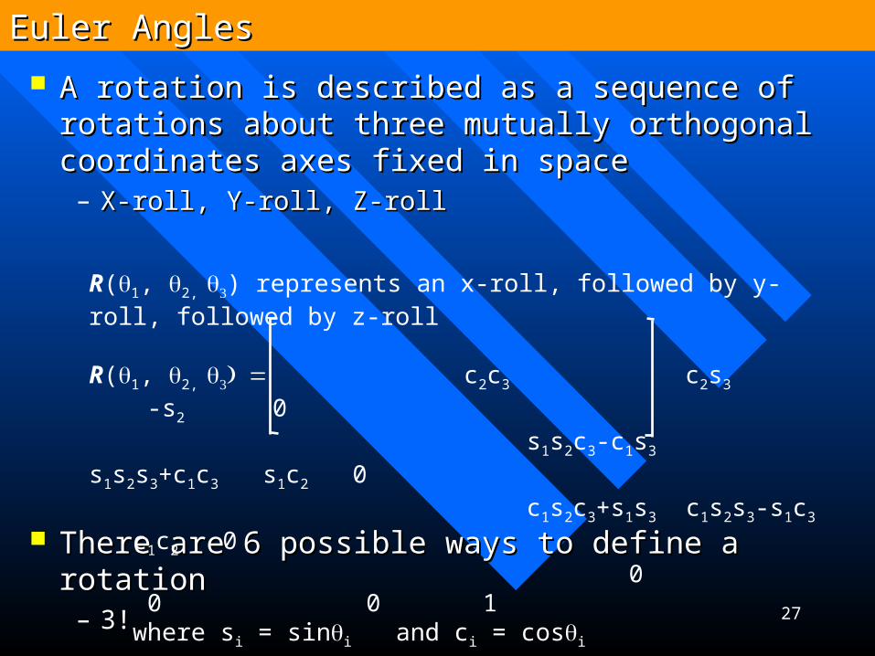
A A rotation is described as a sequence of rotation is described as a sequence of rotations about three mutually orthogonal rotations about three mutually orthogonal coordinates axes fixed in spacecoordinates axes fixed in space– X-roll, X-roll, Y-Y-roll, roll, Z-Z-rollroll
TThere are 6 possible ways to define a rotationhere are 6 possible ways to define a rotation– 3!3!
R(1, 2, ) represents an x-roll, followed by y-roll, followed by z-roll
R(1, 2, c2c3 c2s3 -s2 0 s1s2c3-c1s3 s1s2s3+c1c3 s1c2 0 c1s2c3+s1s3 c1s2s3-s1c3 c1c2 0 0 0 0 1 where si = sini and ci = cosi
Euler AnglesEuler Angles
28
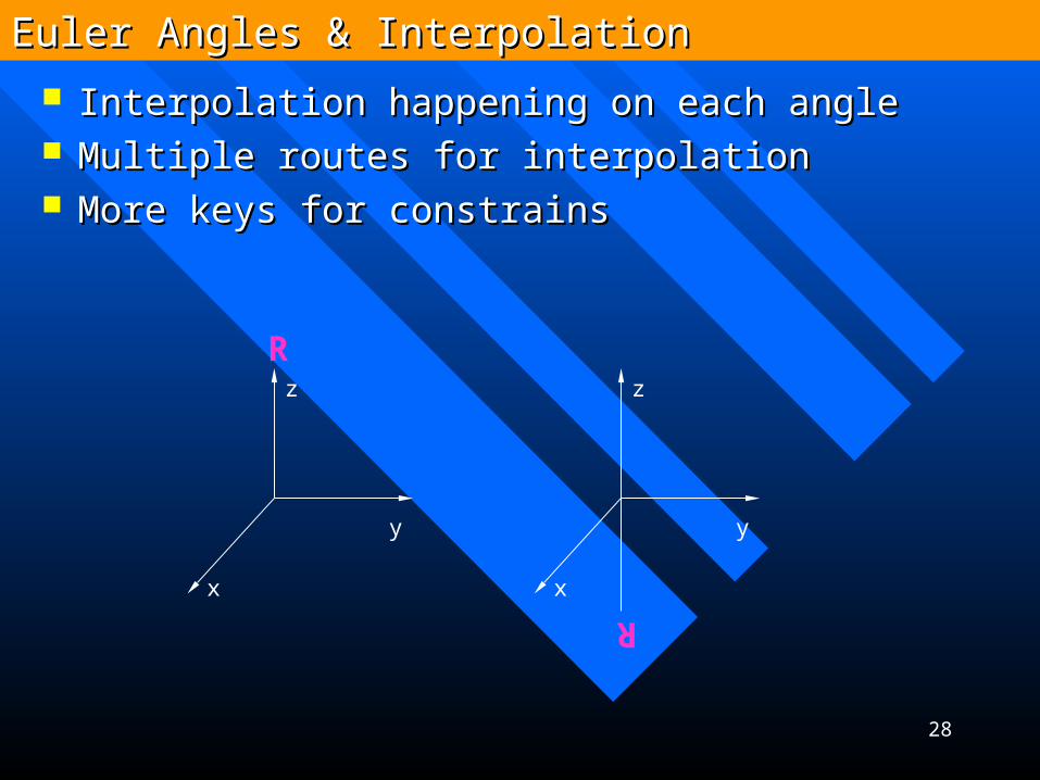
Interpolation happening on each angleInterpolation happening on each angle Multiple routes for interpolationMultiple routes for interpolation MMore keys for constrainsore keys for constrains
z
x
y
Rz
x
y
R
Euler Angles & InterpolationEuler Angles & Interpolation
29
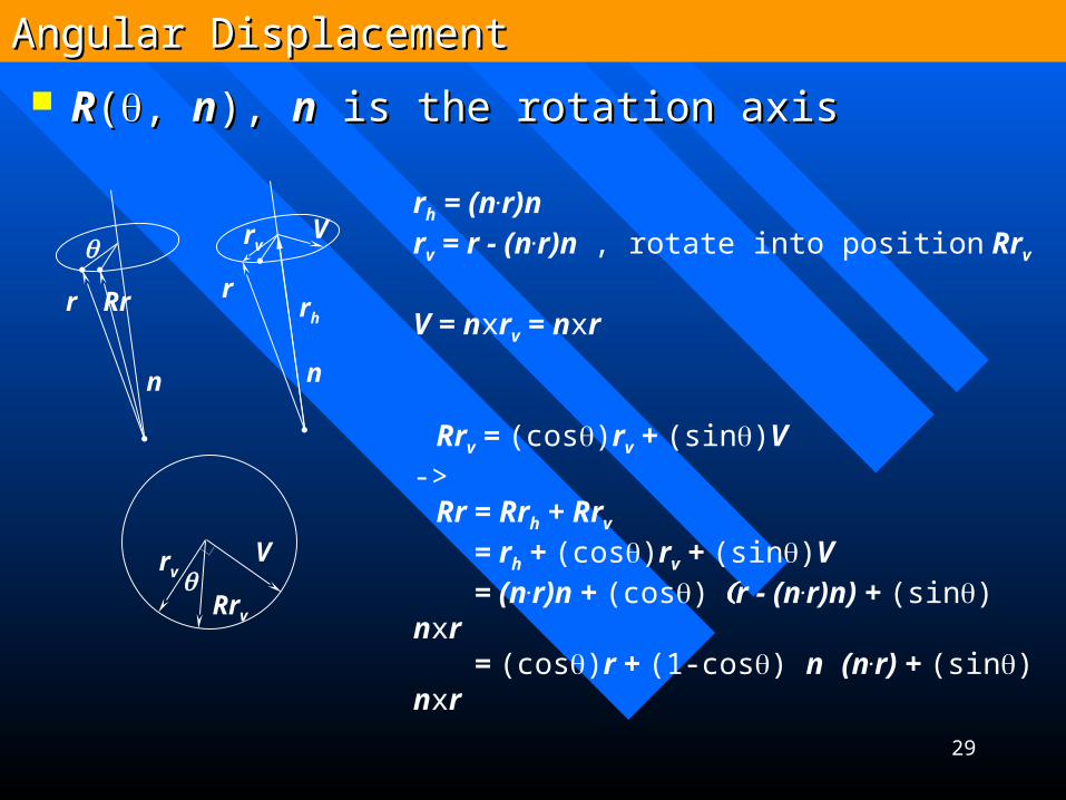
RR((, , nn), ), nn is the rotation axis is the rotation axis
n
r Rr
n
r
rv
rh
V
rv
V
Rrv
rh = (n.r)nrv = r - (n.r)n , rotate into position Rrv
V = nxrv = nxr
Rrv = (cos)rv + (sin)V-> Rr = Rrh + Rrv
= rh + (cos)rv + (sin)V = (n.r)n + (cos)r - (n.r)n) + (sin) nxr = (cos)r + (1-cos) n (n.r) + (sin) nxr
Angular DisplacementAngular Displacement
30
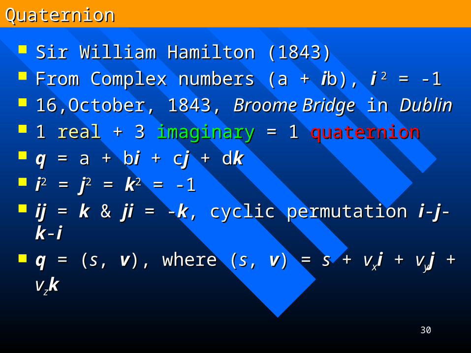
Sir William Hamilton (1843)Sir William Hamilton (1843) FFrom Complex numbers (a + rom Complex numbers (a + iib), b), i i 22 = -1 = -1 16,16,October, 1843, October, 1843, Broome BridgeBroome Bridge in in DublinDublin 1 1 realreal + 3 + 3 imaginaryimaginary = 1 = 1 quaternionquaternion qq = a + b = a + bii + c + cjj + d + dkk ii22 = = jj22 = = kk22 = -1 = -1 ijij = = kk & & jiji = - = -kk, cyclic permutation , cyclic permutation ii--jj--kk--ii qq = ( = (ss, , vv), where (), where (ss, , vv) = ) = ss + + vvxxii + + vvyyjj + + vvzzkk
QuaternionQuaternion
31
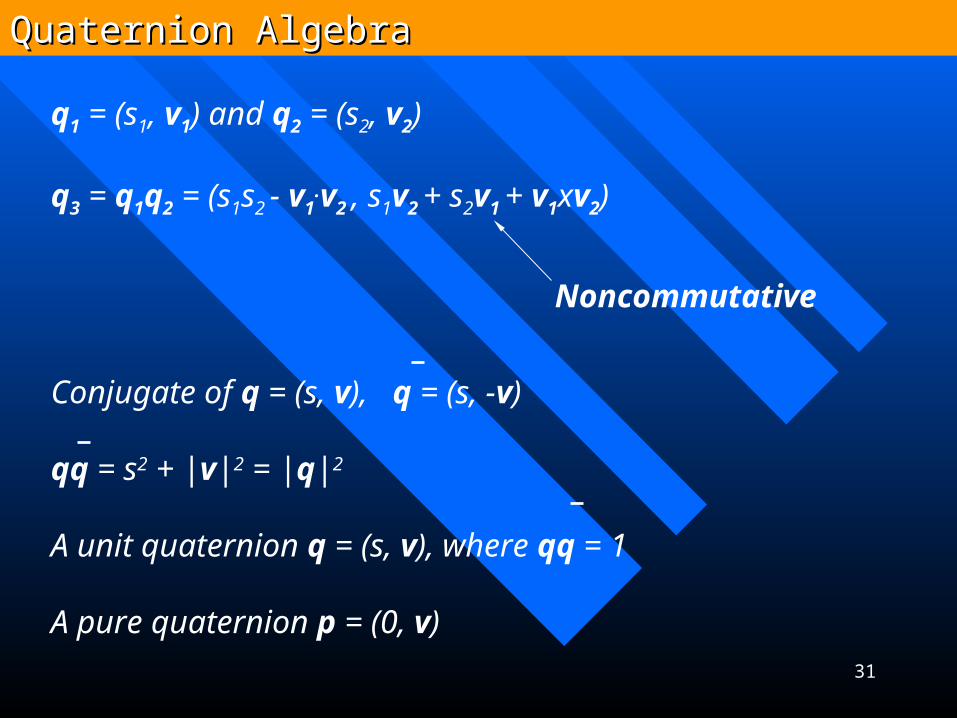
q1 = (s1, v1) and q2 = (s2, v2)
q3 = q1q2 = (s1s2 - v1.v2 , s1v2 + s2v1 + v1xv2)
Conjugate of q = (s, v), q = (s, -v)
qq = s2 + |v|2 = |q|2
A unit quaternion q = (s, v), where qq = 1
A pure quaternion p = (0, v)
Noncommutative
Quaternion AlgebraQuaternion Algebra
32
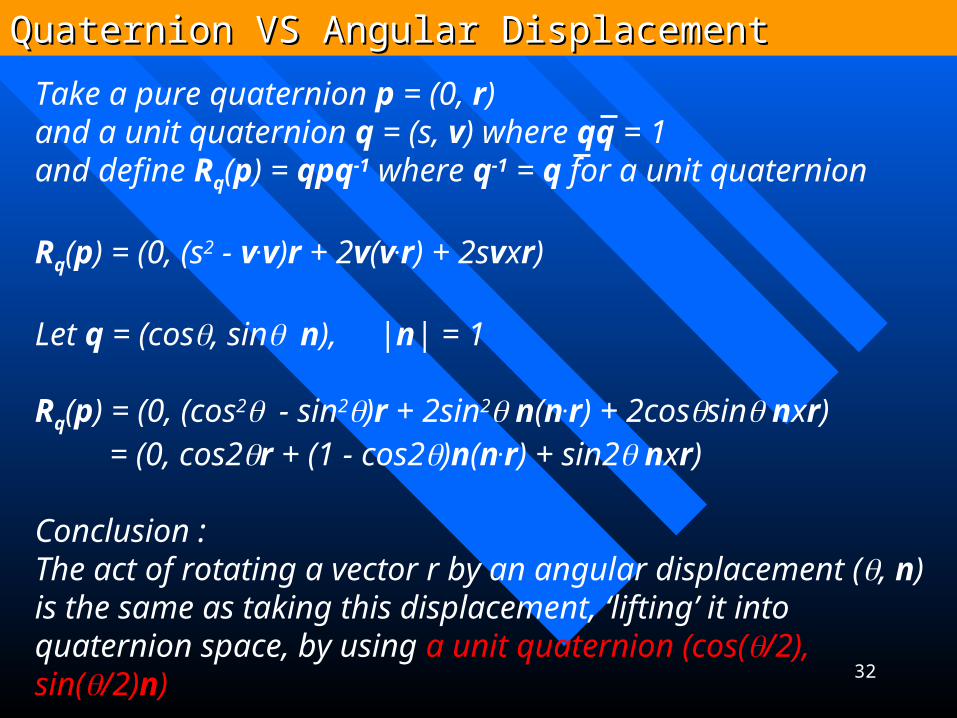
Take a pure quaternion p = (0, r)and a unit quaternion q = (s, v) where qq = 1and define Rq(p) = qpq-1 where q-1 = q for a unit quaternion
Rq(p) = (0, (s2 - v.v)r + 2v(v.r) + 2svxr)
Let q = (cos, sinn), |n| = 1
Rq(p) = (0, (cos2- sin2)r + 2sin2 n(n.r) + 2cossin nxr) = (0, cos2r + (1 - cos2)n(n.r) + sin2 nxr)
Conclusion :The act of rotating a vector r by an angular displacement (, n) is the same as taking this displacement, ‘lifting’ it into quaternion space, by using a unit quaternion (cos(/2), sin(/2)n)
Quaternion VS Angular DisplacementQuaternion VS Angular Displacement
33
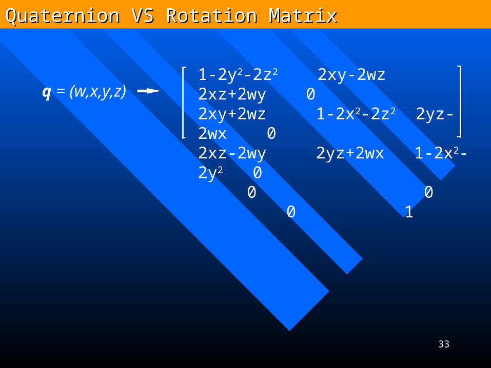
1-2y2-2z2 2xy-2wz 2xz+2wy 02xy+2wz 1-2x2-2z2 2yz-2wx 02xz-2wy 2yz+2wx 1-2x2-2y2 0 0 0 0 1
q = (w,x,y,z)
Quaternion VS Rotation MatrixQuaternion VS Rotation Matrix
34
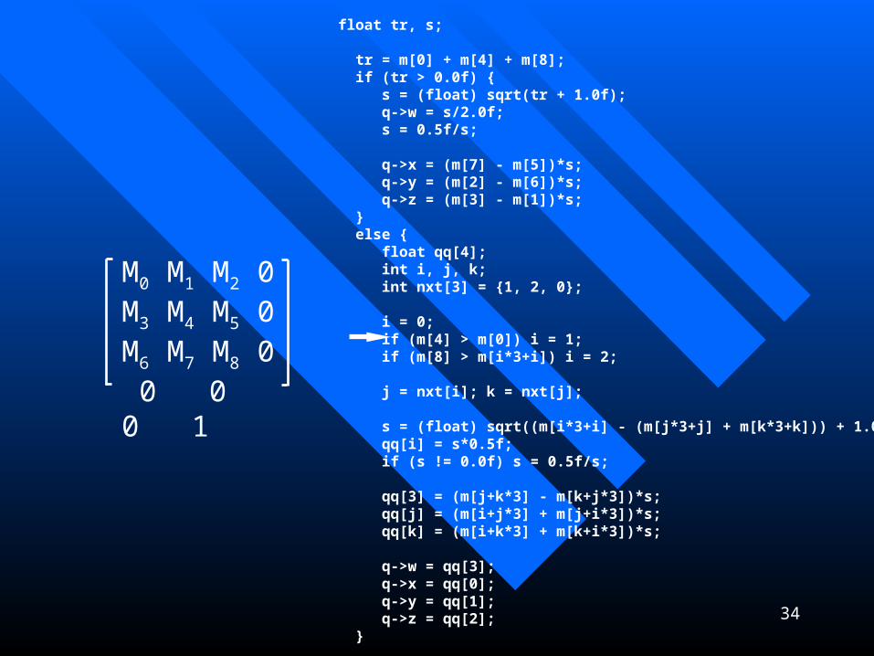
M0 M1 M2 0M3 M4 M5 0M6 M7 M8 0 0 0 0 1
float tr, s;
tr = m[0] + m[4] + m[8]; if (tr > 0.0f) { s = (float) sqrt(tr + 1.0f); q->w = s/2.0f; s = 0.5f/s;
q->x = (m[7] - m[5])*s; q->y = (m[2] - m[6])*s; q->z = (m[3] - m[1])*s; } else { float qq[4]; int i, j, k; int nxt[3] = {1, 2, 0};
i = 0; if (m[4] > m[0]) i = 1; if (m[8] > m[i*3+i]) i = 2;
j = nxt[i]; k = nxt[j];
s = (float) sqrt((m[i*3+i] - (m[j*3+j] + m[k*3+k])) + 1.0f); qq[i] = s*0.5f; if (s != 0.0f) s = 0.5f/s;
qq[3] = (m[j+k*3] - m[k+j*3])*s; qq[j] = (m[i+j*3] + m[j+i*3])*s; qq[k] = (m[i+k*3] + m[k+i*3])*s;
q->w = qq[3]; q->x = qq[0]; q->y = qq[1]; q->z = qq[2]; }
35
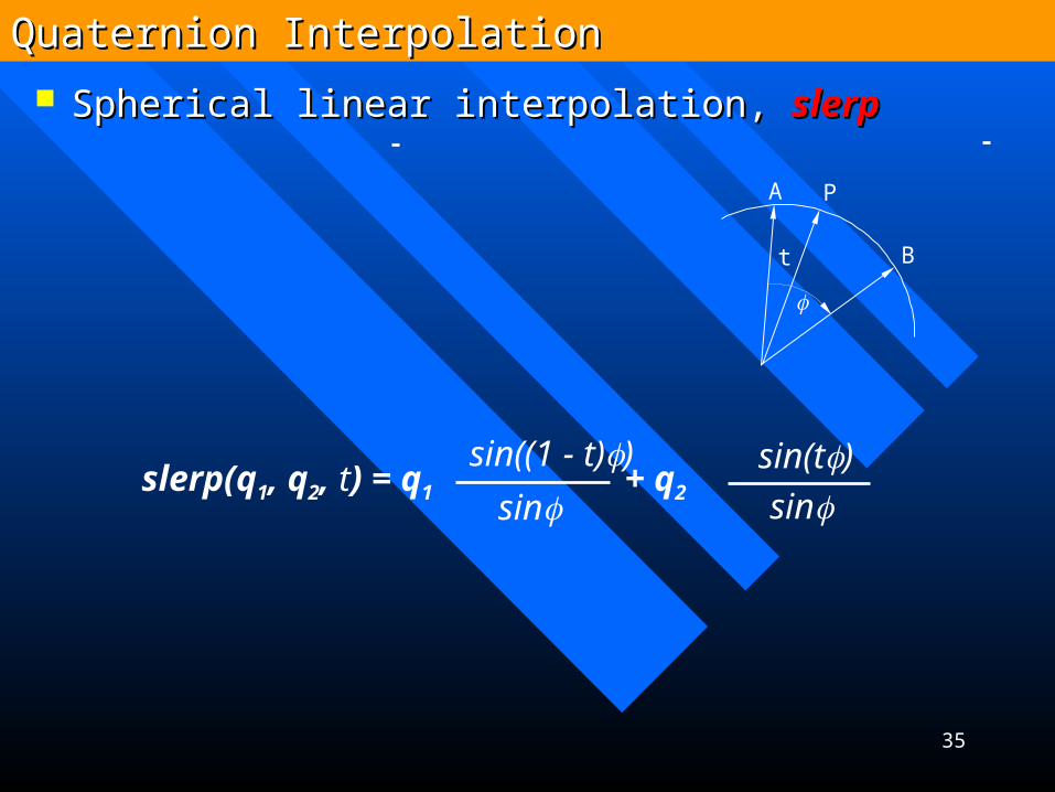
Spherical linear interpolation, Spherical linear interpolation, slerpslerp
A
B
P
t
slerp(q1, q2, t) = q1 + q2
sin((1 - t))
sin sinsin(t)
Quaternion InterpolationQuaternion Interpolation
36
Initial value problemsInitial value problems OODEDE
– Ordinary differential equationOrdinary differential equation
NNumerical solutionsumerical solutions– EEuler’s methoduler’s method– TThe midpoint methodhe midpoint method
Differential Equation BasicsDifferential Equation Basics
37
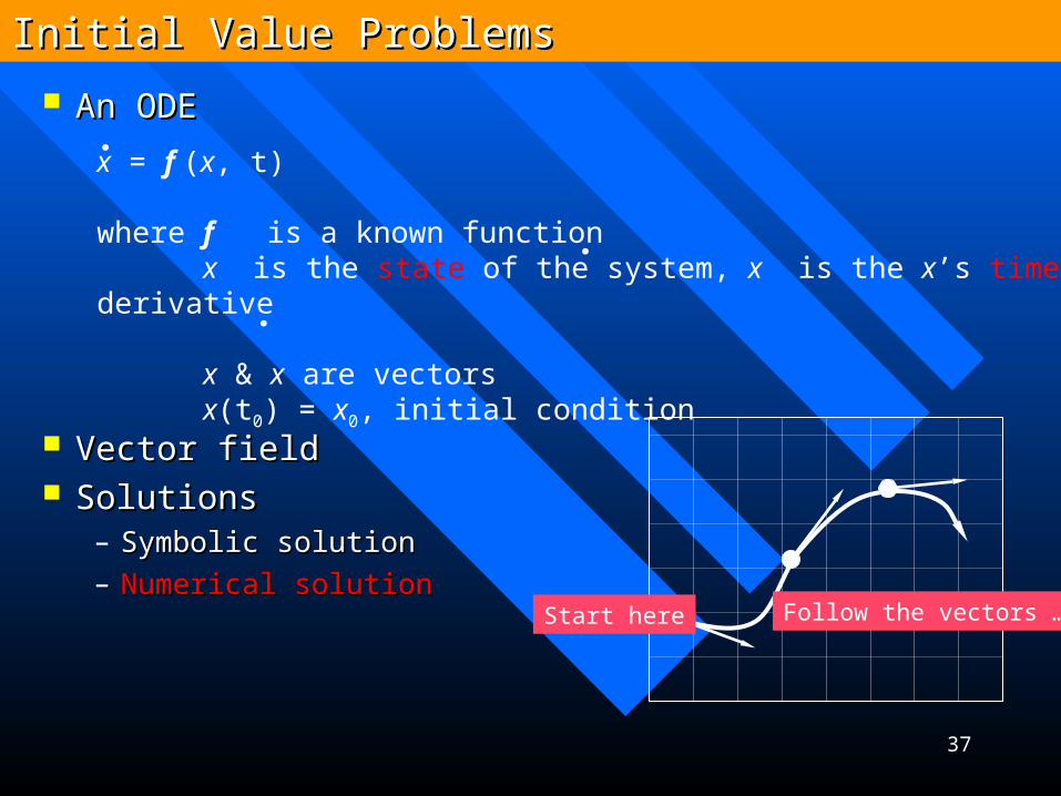
An ODEAn ODE
VVector fieldector field SSolutionsolutions
– SSymbolic solutionymbolic solution– NNumerical solutionumerical solution
x = f (x, t)
where f is a known functionx is the state of the system, x is the x’s time derivative
x & x are vectorsx(t0) = x0, initial condition
.
Start here Follow the vectors …
Initial Value ProblemsInitial Value Problems
.
.

38
A numerical solutionA numerical solution– A simplification from A simplification from Tayler seriesTayler series
DDiscrete time steps starting with initial valueiscrete time steps starting with initial value Simple but not accurateSimple but not accurate
– Bigger steps, bigger errorsBigger steps, bigger errors– OO((tt22) ) errorserrors
Can be unstableCan be unstable Not even efficientNot even efficient
x(t + t) = x(t) + t f(x, t)
Euler’s MethodEuler’s Method
39
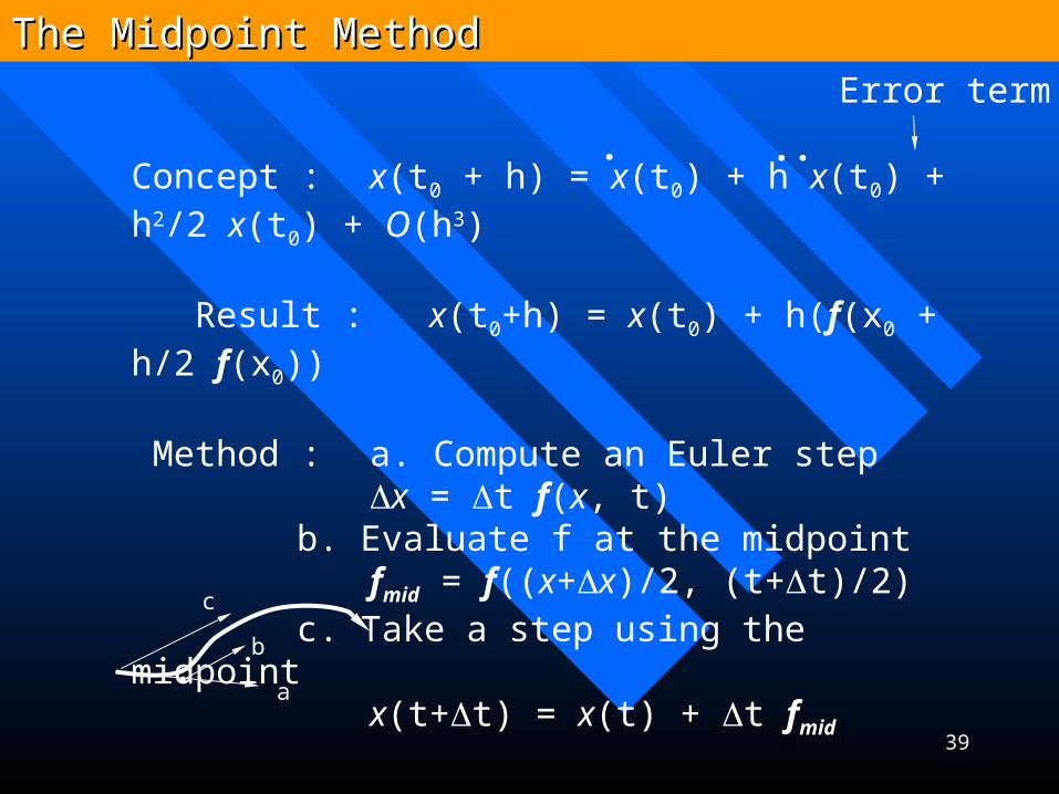
Concept : x(t0 + h) = x(t0) + h x(t0) + h2/2 x(t0) + O(h3)
Result : x(t0+h) = x(t0) + h(f(x0 + h/2 f(x0))
Method : a. Compute an Euler stepx = t f(x, t)
b. Evaluate f at the midpointfmid = f((x+x)/2, (t+t)/2)
c. Take a step using the midpointx(t+t) = x(t) + t fmid
. ..
a
b
c
Error term
The Midpoint MethodThe Midpoint Method
40
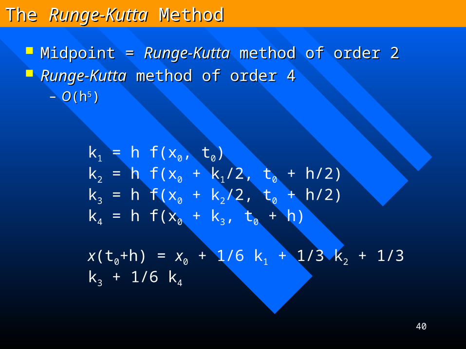
Midpoint = Midpoint = Runge-KuttaRunge-Kutta method of order 2 method of order 2 Runge-KuttaRunge-Kutta method of order 4 method of order 4
– OO(h(h55))
k1 = h f(x0, t0)k2 = h f(x0 + k1/2, t0 + h/2)k3 = h f(x0 + k2/2, t0 + h/2)k4 = h f(x0 + k3, t0 + h)
x(t0+h) = x0 + 1/6 k1 + 1/3 k2 + 1/3 k3 + 1/6 k4
The The Runge-KuttaRunge-Kutta Method Method
41
DynamicsDynamics– Particle systemParticle system
Game FX SystemGame FX System
Initial Value Problems - ApplicationInitial Value Problems - Application
42
Game GeometryGame Geometry
43
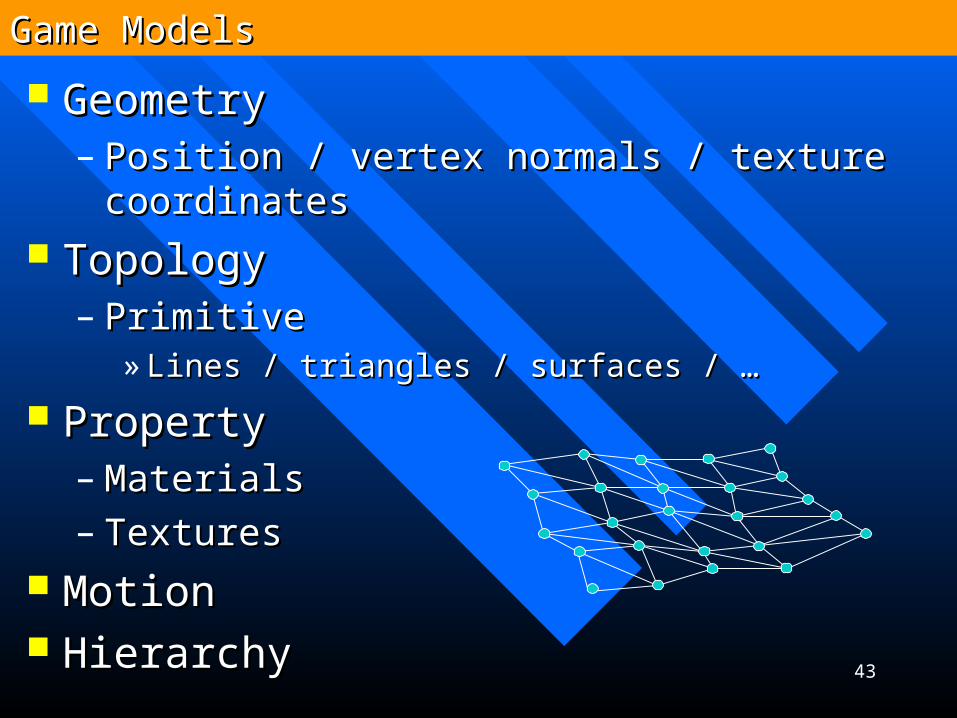
GeometryGeometry– Position / vertex normals / texture Position / vertex normals / texture
coordinatescoordinates TopologyTopology
– PrimitivePrimitive» Lines / triangles / surfaces / …Lines / triangles / surfaces / …
PropertyProperty– MaterialsMaterials– TexturesTextures
MotionMotion HierarchyHierarchy
Game ModelsGame Models
44
Vertex positionVertex position– (x, y, z(x, y, z, w, w))– In model space or screen spaneIn model space or screen spane
Vertex normalVertex normal– (n(nxx, n, nyy, n, nzz))
Vertex colorVertex color– (r, g, b) or (diffuse, specular)(r, g, b) or (diffuse, specular)
Texture coordinates on vertexTexture coordinates on vertex– (u(u11, v, v11), (u), (u22, v, v22), …), …
Skin weightsSkin weights– ((bonebone11, w, w11, bone, bone22, w, w22, …), …)
Geometry DataGeometry Data
45
LinesLines– Line segmentsLine segments– PolylinePolyline
» Open / closedOpen / closed
Indexed trianglesIndexed triangles TTriangle Strips / Fansriangle Strips / Fans SSurfacesurfaces
– NNon-on-uuniform niform RRational ational BB SSpline (pline (NURBSNURBS)) SSubdivisionubdivision
Topology DataTopology Data
46
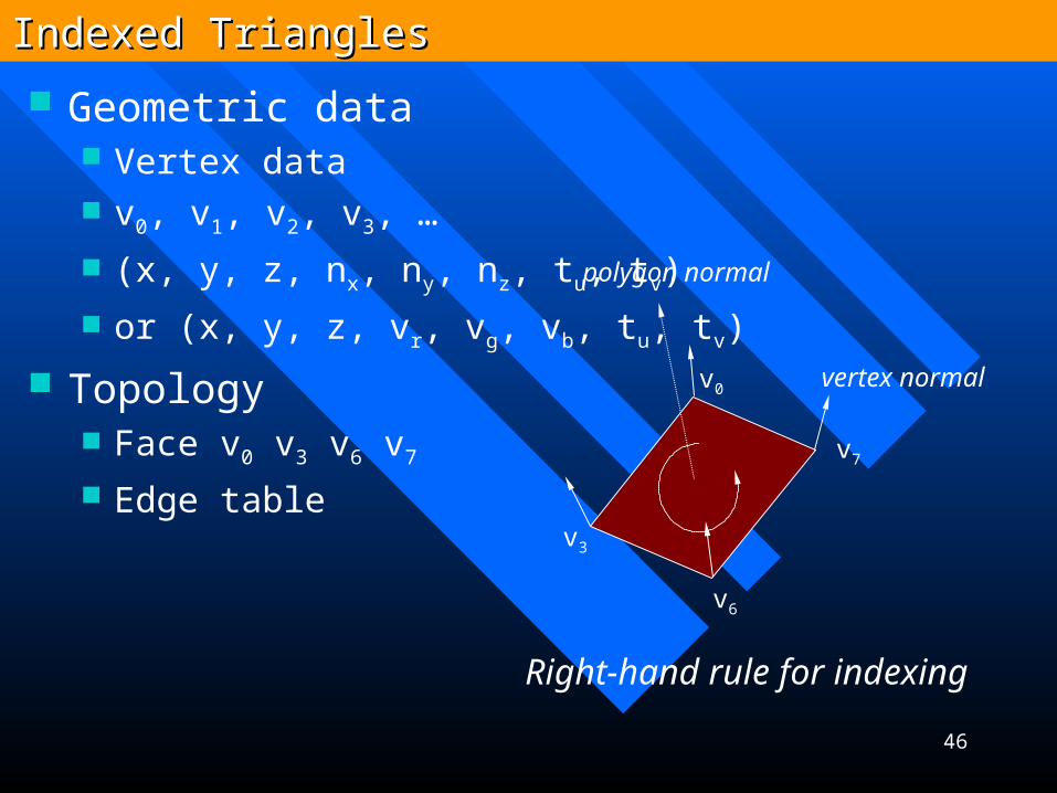
Geometric data Vertex data v0, v1, v2, v3, …
(x, y, z, nx, ny, nz, tu, tv)
or (x, y, z, vr, vg, vb, tu, tv)
Topology Face v0 v3 v6 v7
Edge table
v0
v3
v6
v7
Right-hand rule for indexing
polygon normal
vertex normal
Indexed TrianglesIndexed Triangles
47
v0
v1
v2
v3
v4
v5
v6
v7
T0
T1
T2 T3
T4
T5
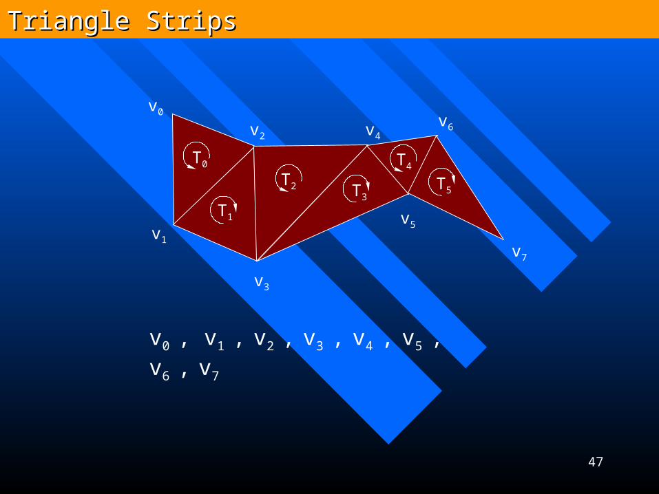
v0 , v1 , v2 , v3 , v4 , v5 , v6 , v7
Triangle StripsTriangle Strips