Embed Size (px)
Citation preview

1
Computer Aided Design
Conf.dr.ing. Ovidiu Pop
2
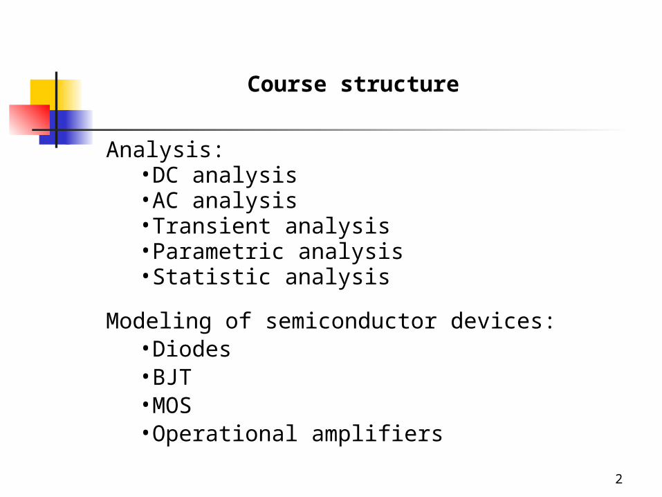
Course structure
Analysis:•DC analysis•AC analysis•Transient analysis•Parametric analysis•Statistic analysis
Modeling of semiconductor devices:•Diodes•BJT•MOS•Operational amplifiers
3
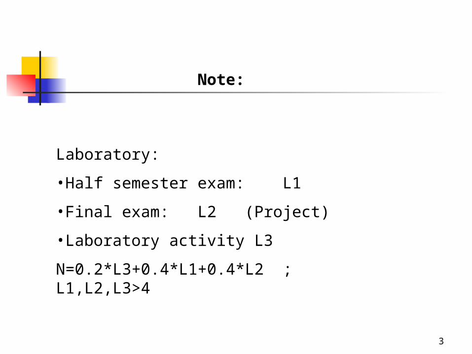
Note:
Laboratory:
•Half semester exam: L1
•Final exam: L2 (Project)
•Laboratory activity L3
N=0.2*L3+0.4*L1+0.4*L2 ; L1,L2,L3>4

4
Minimum Knowledge:
•Editing of electrical circuits
•Primary and Secondary Analysis Categories
•Analysis Settings
•Simulation of circuits
•Interpretation of results

5
INTRODUCTION ON CIRCUIT SIMULATION TECHNIQUES
1. MotivationWhy simulate circuits?
– Design technique of the 50s and 60s:Circuits built-up of discrete elementsExperiments by breadboarding, measuring, tuning
– Later: ICs with growing density of integrationBreadboarding with discrete elements not usefulOnly chip pads accessible for measurementsTime-to-market pressure

6
– test new ideas (‘dry lab’)
– fast changes possible
– considering parasitic effects ( with suitable models)
– simulation of ‘ ideal’ elements (isolation of parasitic components)
– run circuit under conditions which are:
difficult to realize (loading, noise, etc)
dangerous ( destruction of the circuit)
not customary ( needs special equipment)
– fast turnaround
– reduction of costs
What do we gain by simulation?

7
Computer Aided Design CourseCAD
CAD = Computer Aided Drafting , Computer Aided Design
ECAD= Electronic Computer Aided Design
CAE= Computer Aided Engineering
SPICE= Simulation Program with Integrated Circuit Emphasis
PSPICE=Personal Computer SPICE
CAI= Computer Aided Instruction
CAM= Computer Aided Manufacturing
CAP= Computer Aided Planning
CAQ= Computer Aided Quality Control
VLSI IC= Very Large Scale Integration , Integrated Circuit
PLD= Programable Logic Device
ASIC= Application Specific Integrated Circuits
SoC= System On Chip
EDAE= Electronic Design Automation Environment
Glossarry

8
Computer Aided Design CourseCAD
Reference
1. “ECAD Course in Distance Education” Elena Skoikova, Ana Rusu- CDROM, 1999
2. SPICE –User Manual
3. “The SPICE Book “ Andrei Vladimirescu, J. Willey & Sons, 1994
4. “A Guide to Circuit Simulation & Analysis Using PSPICE” P.W. Tuinenga
5. “Semiconductor Device Modeling with SPICE” P. Antognetti, G. Massobrio, McGraw Hill, 1996

9
3. History
50s: development of fundamental knowledge Network description Graph theory State equations
60s: development of first solvers/models/integration algorithms
experience:
-“The first generation simulation programs” (ECAP I in 1965, to IBM) could only solve piecewise linear networks and their scope was fairly limited.
Loop analysis has disadvantages of network contains capacitances and high resistive sources
State equations are not optimal for numerical calculations
70s: application of Nodal Analysis (NA), Modified Nodal Analysis (MNA), Sparse Tableau Analysis (STA);
algorithmic improvements (integration formulas), development of semiconductor models

10
3. History
1971: CANCER, SPICE1, SPICE2 (free distribution)- University of Berkeley“The second generation simulation programs”- Advances in numerical
techniques led in the late 1960s to development of nonlinear analysis programs, such as SPICE1, initially named CANCER (in 1971) to University of Berkeley, California.
80s: SPICE becomes standard simulation tool development of PC versions (1983:PSPICE) commercial versions with better user interface, model support, better stability
and accuraccy integration into CAE design environment
- development of “third generation techniques” for simulation of large-scale circuits. The efforts of three decades ago have crystallized in the two circuit simulators now most often used, SPICE2 and ASTAP, currently called ASX90s: - lot of commercial versions based on SPICE2/ SPICE3
- development of algorithms for very large circuits -versions for multiprocessor systems/supercomputers - development of mixed-signal simulators
2000s: lot of integrated CAD/CAE tools for VLSI submicron circuits

11
4. State of the Art
General-Purpose Circuit Simulators like
SPICE family: SPICE2G.6, HSPICE, PSPICE9 ( from OrCAD, now Cadence), IsSPICE(IntoSoft), AIM-Spice3.2, MicroCapV,
ElectronicWorkBench,…ELDO (mixed-mode) (Anacad, now Mentor)SABER ( mixed-level) (Analogy)
Spectre (Cadence)
Simulators for Special PurposeRF and Microwave (Spectre RF – Cadence, MDS- HP EESoft, Serenade-
AnSoft)Steady State (Oscillator Design)
Symbolic AnalysisMixed-Domain Simulators ( Electro-Thermal, Electro-Mechanical,…)Interconnection AnalysisSignal Integrity
Experimental Simulators ( Univesity, Research Institute) –some may became products
Educational Software
RSPICE, OPTIMA
12
INTRODUCTION TO ELECTRICAL COMPUTER SIMULATION
Knowledge of the behavior of electrical circuits requires the simultaneous solution of a number of equations.
The easiest problem is that of finding the DC operating point of a linear circuit, which requires one to solve a set of equations derived from Kirchhoff’s voltage law and the branch constitutive equations (BCEs).
For a small circuit with linear elements, described by linear branch voltage-current dependencies, the exact DC solution is readily available through hand calculations.
For larger linear circuits the DC solution and especially the frequency-domain or time-domain solutions are very complex.
1. Purpose of Computer Simulation of Electrical Circuits
13
INTRODUCTION TO ELECTRICAL COMPUTER SIMULATION
The analysis of circuits that contain elements described by a nonlinear relation between current and voltage adds another level of complexity, requiring the solution of the nonlinear branch equations simultaneously with the equations based on Kirchhoff ‘s law.
Only small circuits can be solved by hand calculations, which yield only approximate results. Engineers learn in electronics courses to make certain approximations in order to predict the DC operation of small circuits by hand.

14
INTRODUCTION TO ELECTRICAL COMPUTER SIMULATION
Another level of complexity is added when one has to predict the behavior in time or frequency of an electrical circuit.
The nonlinear equations become integro-differential equations, which can be solved by hand only under such approximations as small-signal approximation or other limiting restrictions.

15
Since the electrical design engineer did not have the luxury of a trial-end-error approach in silicon to verify the correctness of the design, a virtual breadboard was needed.
This could be produced on a digital computer by means of an electrical-analysis or simulation program. Programs intended for the electrical analysis of networks without taking any shortcuts in the solution of the KCL, KVL, and BCE equations are called circuit simulators.

16
Another important factor contributing to the development of computer programs for analysis of electrical circuits was the rapidly growth in computers manufacturing.
This two technological factors, ICs and powerful computers, defined both the need and the tool for automating the design process of electronic circuits. A number of researchers started studying the best techniques and algorithms for automating the prediction of the behavior of electric circuits.

17
2. What is SPICE?
SPICE is a general-purpose circuit-simulation program for nonlinear DC, nonlinear transient and linear AC analysis. As outlined above, it solves the network equations for the node voltages. The program is equally suited to solves linear as well as nonlinear electrical circuits.

18
2. What is SPICE?
Circuits can contain:
resistors, capacitors, inductors, mutual inductors, independent voltage and current sources, dependent voltage and current sources, transmission lines, the most common semiconductor devices:
diodes, bipolar junction transistors (BJTs), junction-field effect transistors (JETs), metal-oxide-semiconductor field effect transistors (MOSFETs), metal-semiconductor FETs GaAs (MESFETs); special devices and integrated circuits.
Any general-purpose circuit simulation program must to give the following three basic solutions: bias point (OP), frequency response (AC) and transient response.

19
The DC analysis part of the program computes the bias point of the circuit with capacitors disconnected and inductors short-circuited. SPICE uses iterations to solve the nonlinear network equations; nonlinearities are due mainly to the nonlinear current-voltage (I-V) characteristics of semiconductor devices.
The AC analysis mode computes the complex values of the node voltages of a linear circuit as a function of the frequency of a sinusoidal signal applied at the input. For nonlinear circuits, such as transistor circuits, this type of analysis requires the small-signal assumption; that is, the amplitude of the excitation sources are assumed to be small compared to the thermal voltage for BJTs (Vin
<< Vth= 25mV, for small distortions). Only under this assumption can the nonlinear circuit be replaced by its linearized equivalent around the DC bias point.

20
The transient analysis mode computes the voltage waveforms at each node of the circuit as a function of time. This is a large-signal analysis: no restriction is put on the amplitude of the input signal. Thus the nonlinear characteristics of semiconductor devices are taken into account.
More types of analysis, associated with the above three basic simulation modes, are available in (P)SPICE.
21
WHY USE SPICE?
SPICE is a great tool for learning electronics. You can increase your understanding of circuits as you play and tinker with them.
Experiment! Modify the circuit and see what happens! How long does it take? Change a resistor value and see the effect on a circuit in seconds.
Ideally, we would actually build and test actual circuits to understand all of its behaviors. However, you would need breadboards, components and time to wire the circuit.
22
WHY USE SPICE?
Actual circuits also require expensive equipment like power supplies, signal generators and oscilloscopes. It may be difficult to physically breadboard every circuit you encounter.
You can spend hours building an actual circuit and only get a simple concept from it, whereas, SPICE provides the insight in minutes. SPICE can be your “virtual” breadboard.
Even if you have a short time to spare, you can cover several circuit principles and applications.
23
3. Overview of Simulation Algorithms
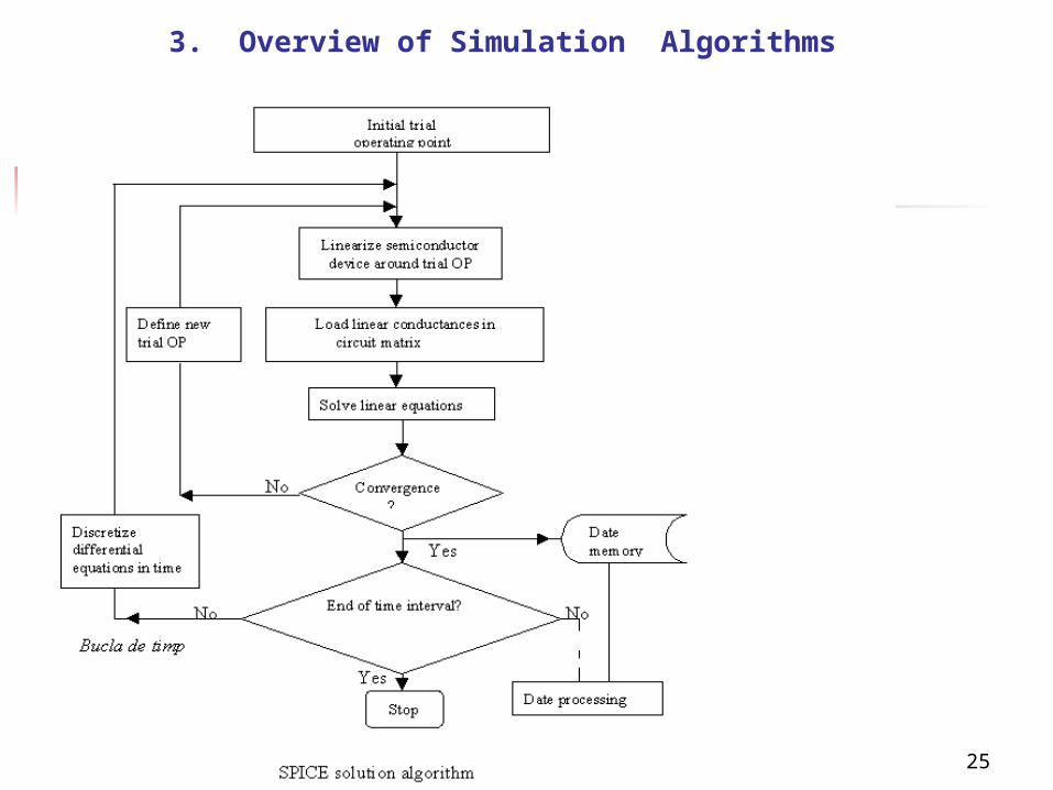
The solution process implemented in SPICE for the time-domain solutions is shown in Fig. 1.
Generally the program first solves for a stable DC operating point. The solution starts with an initial guess of the operating point, which is followed by iterations for solving the DC nonlinear equations.
The iterative process is represented by the inner loop in Fig. 1. The solution the iterative process converges to represents either the small-signal bias solution or the initial transient solution. This is the time zero solution.

24
3. Overview of Simulation Algorithms
The iterative process is repeated for every time point at which the circuit equations are solved in transient analysis.
The time-domain solution uses numerical integration to transform the set of ordinary differential equations (ODEs) into a set of nonlinear algebraic equations.
The time-domain analysis is replaced by a sequence of quasi-static solutions.
25
3. Overview of Simulation Algorithms
26
3. Overview of Simulation Algorithms
A circuit simulator is defined by the following sequence of specific algorithms: (a) an implicit numerical integration method that transforms the nonlinear differential equations into nonlinear algebraic equations; (b) linearization of these through a modified Newton-Raphson iterative algorithm, and finally, (c) Gaussian elimination and sparse matrix techniques that solve the linear equations.
27
4. PSPICE
PSPICE is a mixed analog/digital electrical circuit simulator meaning PSpice can calculate the behavior of analog-only, mixed analog/digital and digital-only circuits with speed and accuracy.
PSpice analog and digital algorithms are build into the same program. Hence, mixed analog/digital circuits can be simulated with tightly-coupled feedback loops between the analog and digital sections, without any performance degradation.
PSpice calculates “voltage” and “currents” of the analog components and nodes, and “states” of the nodes connected to digital components. The results are formulated into meaningful graphical traces, tables and plots for further analysis.

28
4. PSPICE
Literal numeric values are written in standard floating point notation.
PSpice assumes default units for numbers described component values and electrical quatities. However, values can be scaled by following the number by the appropriate scale suffix as shown in Table 1.
Numeric values can also be indirectly represented by parameters (PARAM) Numeric values and parameters can be used together to form arithmetic expressions. PSpice expressions may incorporate the intrinsic functions (ABS, SQRT, EXP, LOG, LOG10, PWR, SIN, COS, TAN, ATAN, TABLE, LIMIT) and user-functions (FUNC).
4.1. Numeric Value and Expression

29
Table 1. Scale suffixes for numeric values
30
Elements and models/macromodels description represents the core of the circuit description.
An element statement (in netlist file) contains connectivity information (circuit topology from schematics) and either explicity or by reference to a model/subcircuit name (from a models library), the value of the defined element.
Model (MODEL)/macromodel (SUBCKT) statements are necessary for defining the parameters of complex elements: all semiconductor devices and many ICs.
2.Elements, Models and Nodes

31

32
33
4.3. Conventions
The following conventions must be observed in the circuit definitions:
A circuit must always contain a ground node, which must always be number 0.
Every node in the circuit must have at least two elements connected to it; the only exceptions are the nodes of unterminated transmission lines.
Every node in the circuit must have a DC path to ground. In DC, capacitors represent open circuits and inductors represent shorts. This requirement prevents the occurrence of floating nodes, for which the program cannot find a bias point.

34
Because standard SPICE2G.6 uses modified nodal analysis to solve for both node voltages and currents of voltage-defined elements, such as voltage sources and inductors, two restrictions must be observed:
the circuit cannot contain a loop of voltage sources or inductors
it cannot contain a cut-set of current sources or capacitors.
The former is disallowed due to Kirchhoff’s voltage law and the latter due to Kirchhoff’s current law.

35
Any violation of the above restrictions results in an error message and termination of the SPICE program. The possible error messages and corrective actions are:
During read-in, PSpice checks the topology of the circuit. One of the checks done is to make sure that there are no floating nodes. If there are floating nodes, PSpice will indicate a read-in error on the screen and the output file will contain a message similar to the following:
ERROR: Node X is floating.
This means that there is no DC path to ground from node X. A DC path is one that draws current, for instance a path through resistors, inductors and transistors. There are several paths that do not draw current and that do not count:
The two ends of a transmission line do not have a DC connection between them: in the following example node 5 has a connection to node 0 (ground):
T1 5 0 4 8 Z0=75 td=20ns
1. “Floating Nodes”
36
Voltage-controlled sources do not have a DC connection to their controlling nodes, so these sources do not draw current from their controlling nodes. In the following examples, node 5 has a connection to ground:
EGAIN 5 0 4 8 100GA 5 0 4 8 0.8
The two sides of a capacitor have no DC connection between them. In the following example, node 5 has no DC path to ground:
C5 5 0 0.1uIn all these cases the solution is straightforward: connect the floating circuitry to ground with a resistor (usually of large value, 1MEGohm).

37
Another topology check that is done on each circuit is to make sure that there are no loops with zero resistance. If there are, PSpice will indicate a read-in error on the screen and the output file will contain a message similar to the following:
ERROR: Voltage loop involving VxThis means that the circuit has a loop of zero resistance
components, one of which is Vx.The zero resistance components in PSpice are: independent voltage
sources (V), inductors (L), voltage-controlled voltage sources (E), and current-controlled voltage source (H). Examples of such loops are:a.) Vin 3 0 10V
Vs 3 0 5Vb.) V1 3 5 15V
L1 3 5 10uE1 3 5 2 7 10
2. “Voltage Source/Inductor Loop”

38
Note that it makes no difference whether the values of the voltage sources are 0 or not. Having a zero resistance loop means that the program will need to divide 10V ( or any value of voltage) by 0, which is impossible.
In all these cases the solution is straighforward: add a series resistance to at least one component in the loop. Choose the resistor’s value to be small enough so that it does not disturb the operation of the circuit. However, to avoid exceeding the dynamic range of the double-precision arithmetic used in PSpice, it is recommended not going bellow 1micro-ohm. To be more accurate, choose a value that approximates the actual parasitic resistance of the component.
39
During the read-in and checking part of a run you may get an error which prints the message in the output file:
ERROR: Less than 2 connections at node XThe inputs to voltage-controlled sources are not considered
connections during this check. This is because these inputs are ideal inputs and draw no current (they have infinite impedance).If this occurs, the solution is: connect a very large resistor (a Gohms, say) from the source’s input to ground. This will satisfy the topology check and, if the resistor is large enough it will not affect the circuit’s behavior.
3.“Voltage-Controlled Sources”

40
The DC sweep, bias point calculation and transient analysis all use iterative algorithms.
These algorithms start with a set of node voltages and for each iteration they calculate a new set of node voltages which hopefully are closer to a solution of Kirchhoff’s voltage and current laws. In other words, an initial guess is used and successive iterations are supposed to converge to the solution.
If the iterations do not converge onto a solution, then the analysis fails. The DC sweep skips the remaining points in the sweep. Failure of the bias-point calculation prevents other analyses (AC, sensitivity, etc) which depend on it from being done. The transient analysis skips the remaining time.
4.4. Convergence Problems

41
The DC sweep skips the remaining points in the sweep. Failure of the bias-point calculation prevents other
analyses (AC, sensitivity, etc) which depend on it from being done.
The transient analysis skips the remaining time.
PSpice is successful in analyzing most circuits. Considerable effort has gone into eliminating problems which impeded the progression of circuit analysis. However, there are no guarantees. If an analysis fails for our circuit, the company give us few suggestions for: DC Sweep analysis, Bias Point, Transient Analysis.
4.4. Convergence Problems