Embed Size (px)
Citation preview
1
Chapter 5 Laplace Transform5.1 Introduction
( ) ( , ) ( )b
aF s K t s f t dt
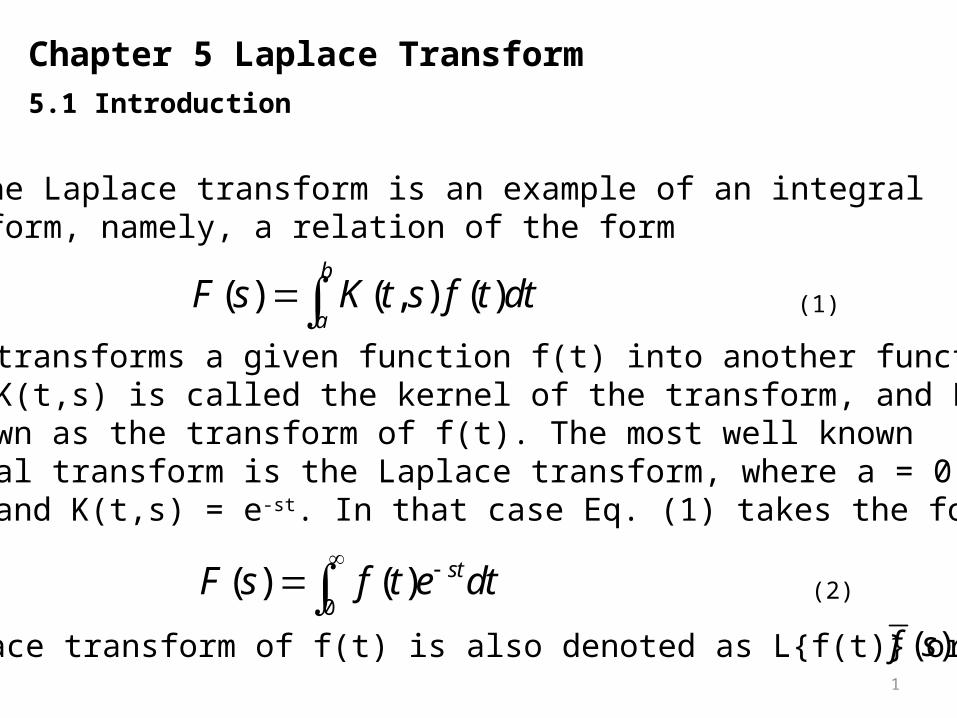
The Laplace transform is an example of an integral transform, namely, a relation of the form
(1)
0( ) ( ) stF s f t e dt
which transforms a given function f(t) into another function F(s); K(t,s) is called the kernel of the transform, and F(s) is known as the transform of f(t). The most well known Integral transform is the Laplace transform, where a = 0, b =∞, and K(t,s) = e-st. In that case Eq. (1) takes the form
(2)
The Laplace transform of f(t) is also denoted as L{f(t)} or as .( )f s
2
The basic idea behind any transform is that the given problem can be solved more readily in the “transform domain”. In this chapter, we use t as the independent variable and consider the interval 0 t <∞ because in most applications of the Laplace ≦transform the independent variable is the time t, with 0 t <∞. ≦
5.2 Calculation of the Transform
5.3Properties of the transform
5.4 Application to the solution of differential equations
5.5 Discontinuous forcing functions; Heaviside step function
5.6 Impulsive forcing function; Diarac impulse function
5.7 Additional properties
3
0( ) ( ) stF s f t e dt
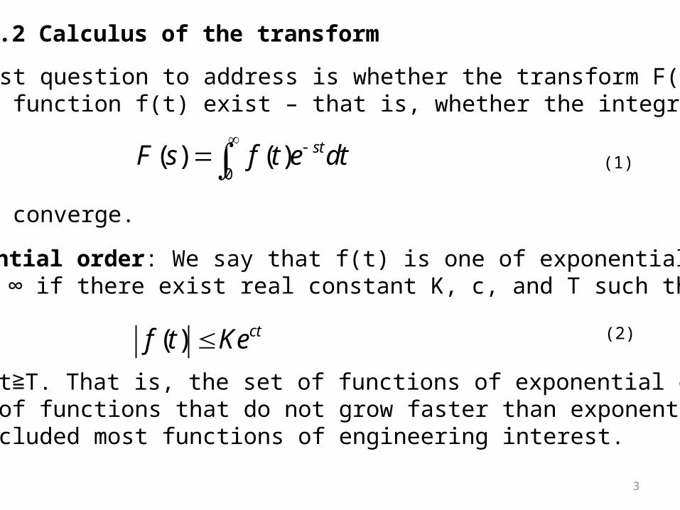
5.2 Calculus of the transform
The first question to address is whether the transform F(s) of a given function f(t) exist – that is, whether the integral
(1)
converge.
Exponential order: We say that f(t) is one of exponential order as t → ∞ if there exist real constant K, c, and T such that
( ) ctf t Ke (2)
For all t T. That is, the set of functions of exponential order is ≧the set of functions that do not grow faster than exponentially, which included most functions of engineering interest.
4
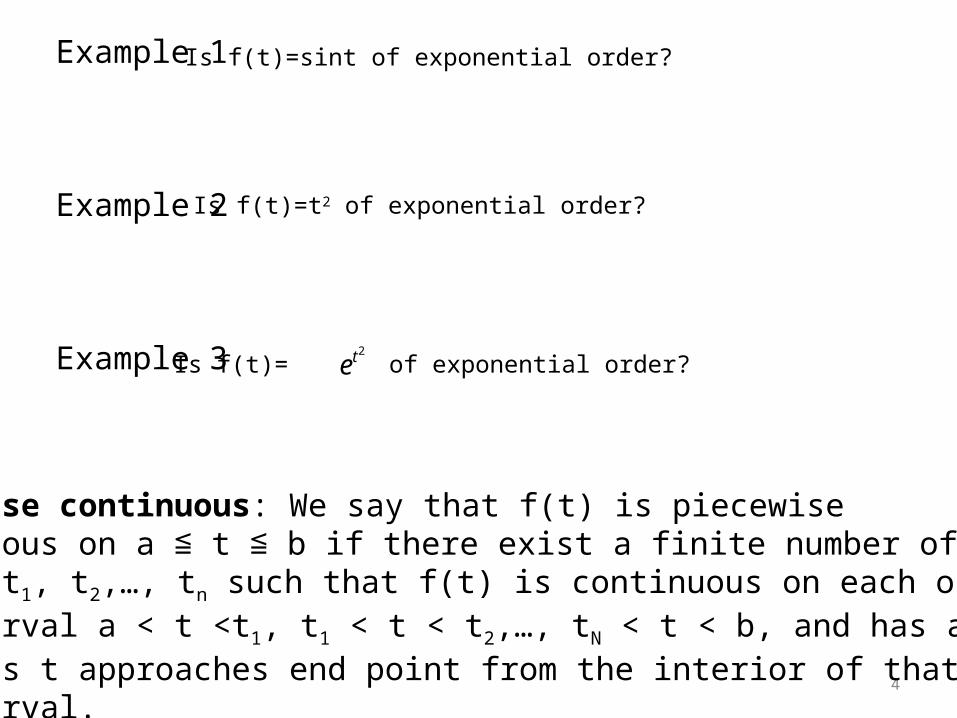
Example 1
Example 2
Example 3
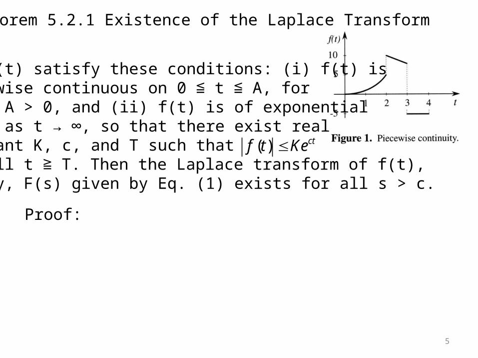
Piecewise continuous: We say that f(t) is piecewise continuous on a t b if there exist a finite number of ≦ ≦points t1, t2,…, tn such that f(t) is continuous on each open subinterval a < t <t1, t1 < t < t2,…, tN < t < b, and has a finite limit as t approaches end point from the interior of that subinterval.
Is f(t)=sint of exponential order?
Is f(t)=t2 of exponential order?
Is f(t)= of exponential order?2te
5
Theorem 5.2.1 Existence of the Laplace Transform
Let f(t) satisfy these conditions: (i) f(t) is piecewise continuous on 0 t A, for ≦ ≦every A > 0, and (ii) f(t) is of exponential order as t → ∞, so that there exist real constant K, c, and T such thatfor all t T. Then the Laplace transform of f(t), ≧namely, F(s) given by Eq. (1) exists for all s > c.
( ) ctf t Ke
Proof:
6
Example 4 Find the Laplace transform of f(t) = 1
Example 5 Find the Laplace transform of f(t) = eat
Example 6 Find the Laplace transform of f(t) = sinat
7
Example 7 Find the Laplace transform of f(t) =
Example 8 Find the Laplace transform of f(t) =sinhat
1
t
For more information on the Laplace transform, please see Laplace transform table in Appendix C. (p. 1271)
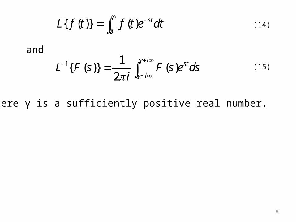
Define Laplace transform operator L and inverse transform operator L-1 as:
8
0{ ( )} ( ) stL f t f t e dt
and
1 1{ ( )} ( )
2
i st
iL F s F s e ds
i
(14)
(15)
Where γ is a sufficiently positive real number.
9
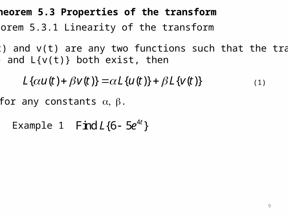
Theorem 5.3 Properties of the transform
Theorem 5.3.1 Linearity of the transform
Let u(t) and v(t) are any two functions such that the transforms L{u(t)} and L{v(t)} both exist, then
{ ( ) ( )} { ( )} { ( )}L u t v t L u t L v t (1)
for any constants .
Example 1 4Find {6 5 }tL e
10
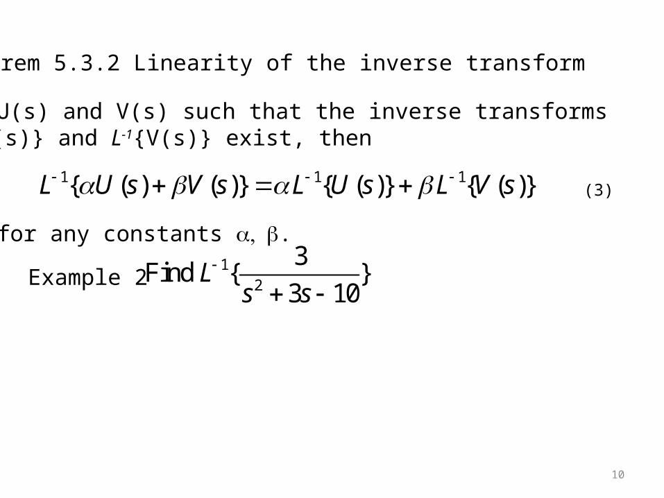
Theorem 5.3.2 Linearity of the inverse transform
Let U(s) and V(s) such that the inverse transforms L-1{U(s)} and L-1{V(s)} exist, then
1 1 1{ ( ) ( )} { ( )} { ( )}L U s V s L U s L V s (3)
for any constants .
Example 21
2
3Find { }
3 10L
s s
11
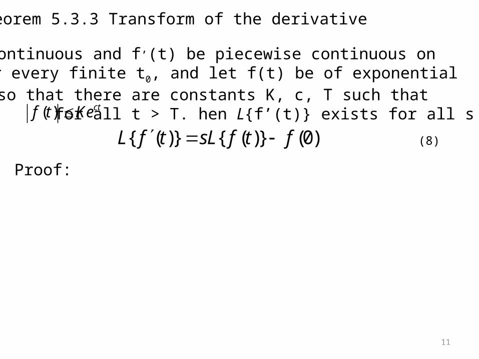
Theorem 5.3.3 Transform of the derivative
Let f(t) be continuous and f’(t) be piecewise continuous on0 t t≦ ≦ 0 for every finite t0, and let f(t) be of exponential order as t→∞ so that there are constants K, c, T such that for all t > T. hen L{f’(t)} exists for all s > c, and
{ ( )} { ( )} (0)L f t sL f t f (8)
( ) ctf t Ke
Proof:
12
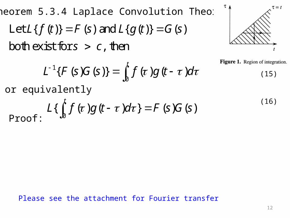
Theorem 5.3.4 Laplace Convolution Theorem
Let { ( )} ( ) and { ( )} ( )
both exist for , then
L f t F s L g t G s
s c
(15)
Proof:
1
0{ ( ) ( )} ( ) ( )
tL F s G s f g t d
or equivalently
0{ ( ) ( ) } ( ) ( )
tL f g t d F s G s
(16)
Please see the attachment for Fourier transfer
13
Example 3
Example 4
12
3Find
3 10L
s s
0Find ( ) cos3( - )
tf t t d
14
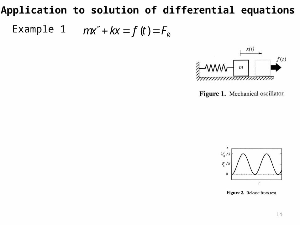
5.4 Application to solution of differential equations
Example 10( )mx kx f t F
15
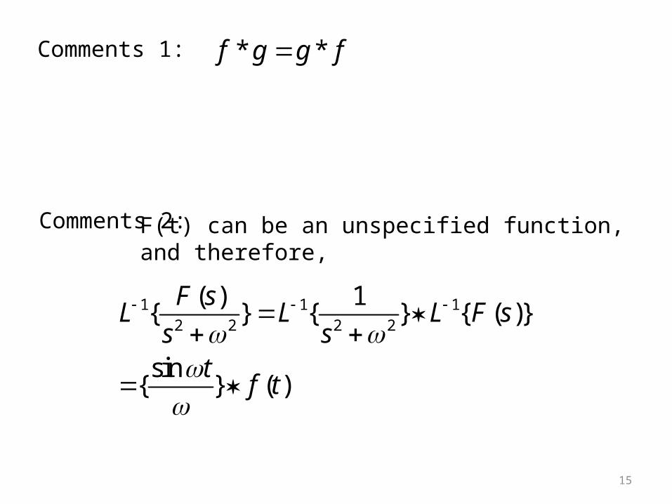
Comments 1: * *f g g f
Comments 2: F(t) can be an unspecified function, and therefore,
1 1 12 2 2 2
( ) 1{ } { } { ( )}
sin{ } ( )
F sL L L F s
s st
f t
16
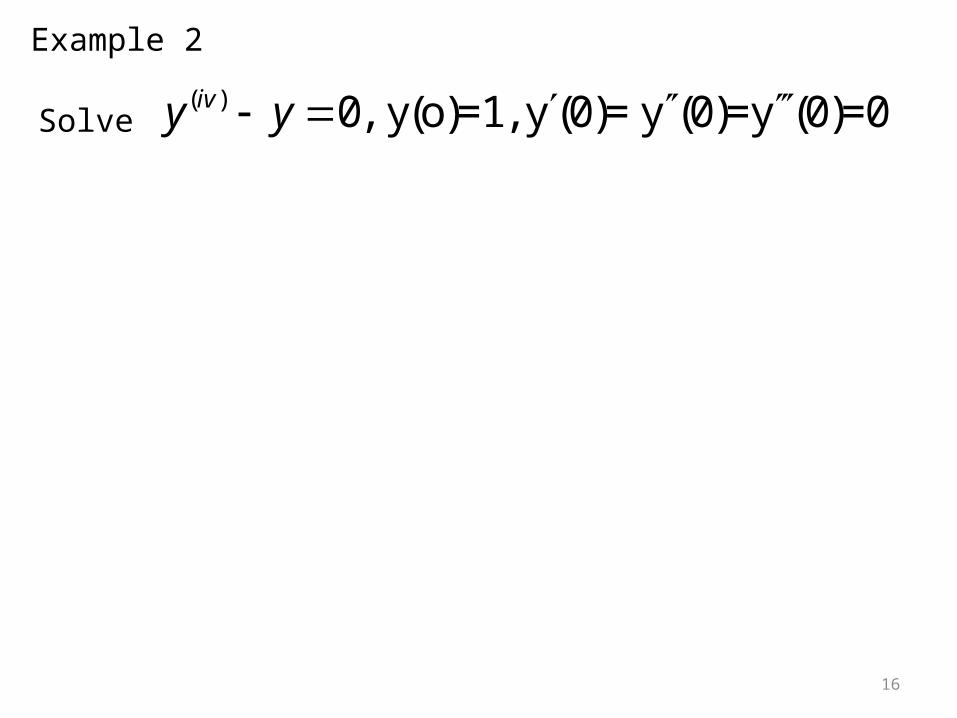
Example 2
Solve ( ) 0, y(o)=1, y (0)= y (0)=y (0)=0ivy y
17
Example 3
0( ) x(0)=xx px q t Solve
18
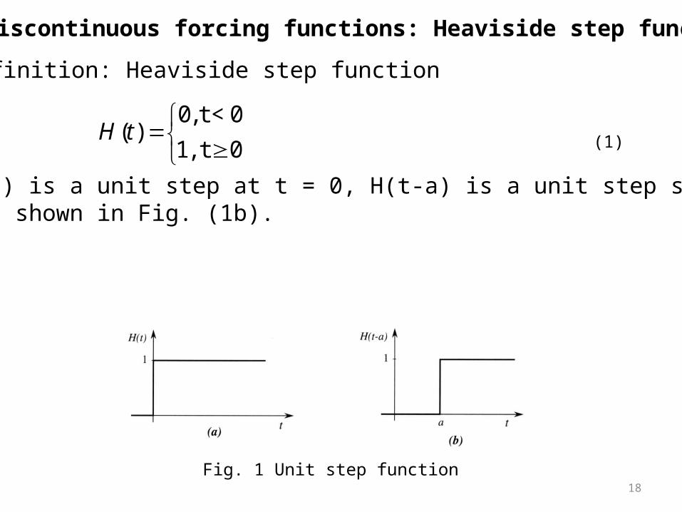
5.5 Discontinuous forcing functions: Heaviside step function
Definition: Heaviside step function
0, t < 0( )
1, t 0H t
(1)
Since H(t) is a unit step at t = 0, H(t-a) is a unit step shifted to t = a, shown in Fig. (1b).
Fig. 1 Unit step function
19
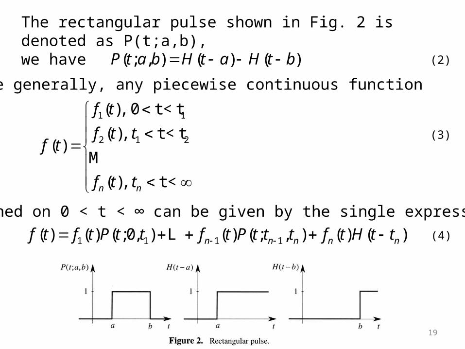
More generally, any piecewise continuous function
1 1
2 1 2
( ), 0 t < t
( ), t < t( )
( ), t < n n
f t
f t tf t
f t t
M
(3)
defined on 0 < t < ∞ can be given by the single expression
1 1 1 1( ) ( ) ( ;0, ) ( ) ( ; , ) ( ) ( )n n n n nf t f t P t t f t P t t t f t H t t L (4)
The rectangular pulse shown in Fig. 2 is denoted as P(t;a,b), we have
( ; , ) ( ) ( )P t a b H t a H t b (2)
20
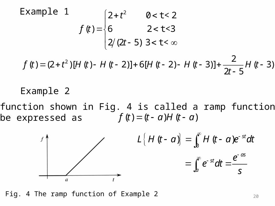
Example 1 22 0 t < 2
( ) 6 2 t <3
2 (2 5) 3 t <
t
f t
t
2 2( ) (2 )[ ( ) ( 2)] 6[ ( 2) ( 3)] ( 3)
2 5f t t H t H t H t H t H t
t
Example 2
The function shown in Fig. 4 is called a ramp function which can be expressed as ( ) ( ) ( )f t t a H t a
Fig. 4 The ramp function of Example 2
0
( ) ( )
st
asst
a
L H t a H t a e dt
ee dt
s
21
( )ase
L H t as
(8)
( ) ( ) ( )asL H t a f t a e F s (9)
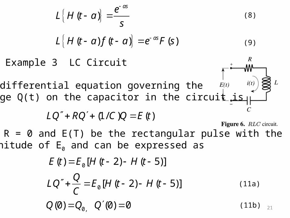
Example 3 LC Circuit
The differential equation governing the charge Q(t) on the capacitor in the circuit is
(1/ ) ( )LQ RQ C Q E t
Let R = 0 and E(T) be the rectangular pulse with the magnitude of E0 and can be expressed as
0( ) [ ( 2) ( 5)]E t E H t H t
(11a)
(11b)
0[ ( 2) ( 5)]Q
LQ E H t H tC
0, (0) (0) 0Q Q Q
22
0{ } { [ ( 2) ( 5)]}Q
L LQ L E H t H tC
23
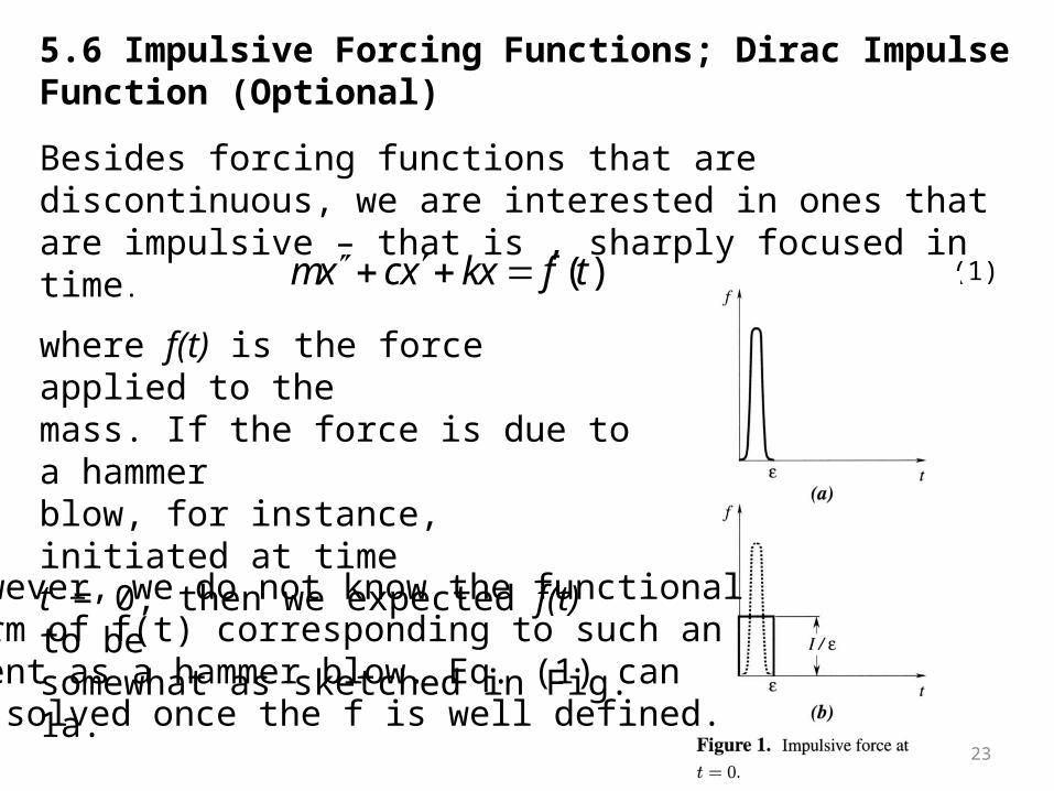
Besides forcing functions that are discontinuous, we are interested in ones that are impulsive – that is , sharply focused in time.
5.6 Impulsive Forcing Functions; Dirac Impulse Function (Optional)
where f(t) is the force applied to the mass. If the force is due to a hammer blow, for instance, initiated at time t = 0, then we expected f(t) to be somewhat as sketched in Fig. 1a.
( )mx cx kx f t (1)
However, we do not know the functional form of f(t) corresponding to such an event as a hammer blow. Eq. (1) can be solved once the f is well defined.
24
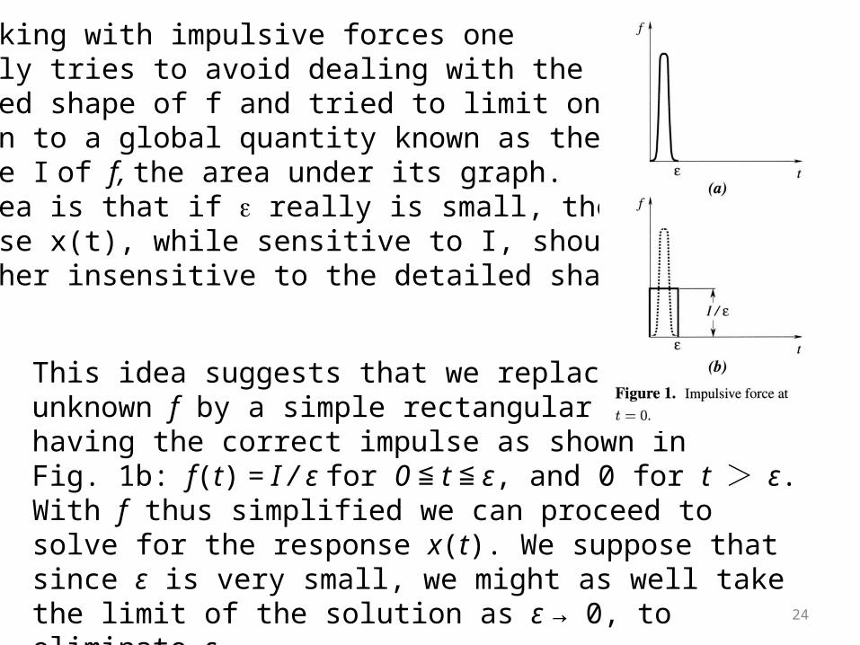
This idea suggests that we replace the unknown f by a simple rectangular pulse having the correct impulse as shown in Fig. 1b: f(t) = I / ε for 0 ≦ t ≦ ε, and 0 for t > ε. With f thus simplified we can proceed to solve for the response x(t). We suppose that since ε is very small, we might as well take the limit of the solution as ε → 0, to eliminate ε.
In working with impulsive forces one normally tries to avoid dealing with the detailed shape of f and tried to limit one’s concern to a global quantity known as the impulse Ι of f, the area under its graph. The idea is that if really is small, then the response x(t), while sensitive to I, should be rather insensitive to the detailed shape of f.
25
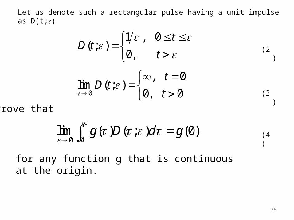
Let us denote such a rectangular pulse having a unit impulse as D(t;)
0
, 0lim ( ; )
0, 0
tD t
t
00lim ( ) ( ; ) (0)g D d g
Prove that
(2)
(4)
1 , 0( ; )
0,
tD t
t
(3)
for any function g that is continuous at the origin.
26
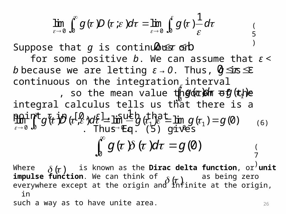
Where is known as the Dirac delta function, or unit impulse function. We can think of as being zeroeverywhere except at the origin and infinite at the origin, in such a way as to have unite area.
0 00 0
1lim ( ) ( ; ) lim ( )g D d g d
10( ) ( )g d g
0( ) ( ) (0)g d g
( ) ( )
(5)
Suppose that g is continuous on for some positive b. We can assume that ε < b because we are letting ε → 0. Thus, g is continuous on the integration interval , so the mean value theorem of the integral calculus tells us that there is a point τ1 in [0, ε], such that . Thus Eq. (5) gives
0 b
0 ε
(7)
1 100 0 0
1lim ( ) ( ; ) lim ( ) lim ( ) (0)g D d g g g
(6)
27
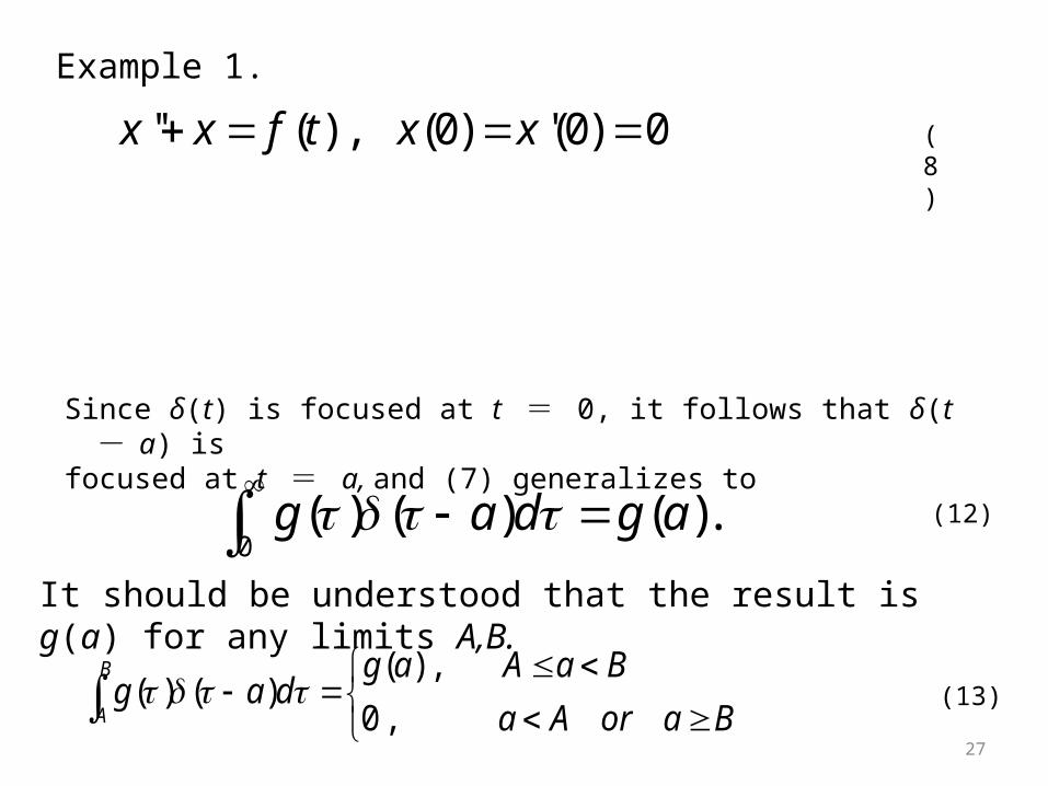
Since δ(t) is focused at t = 0, it follows that δ(t - a) is focused at t = a, and (7) generalizes to
'' ( ) , (0) '(0) 0x x f t x x
BaorAa
BaAagdag
B
A ,0
,)()()(
Example 1.
(8)
(12)
It should be understood that the result is g(a) for any limits A,B.
0( ) ( ) ( ).g a d g a
(13)
28
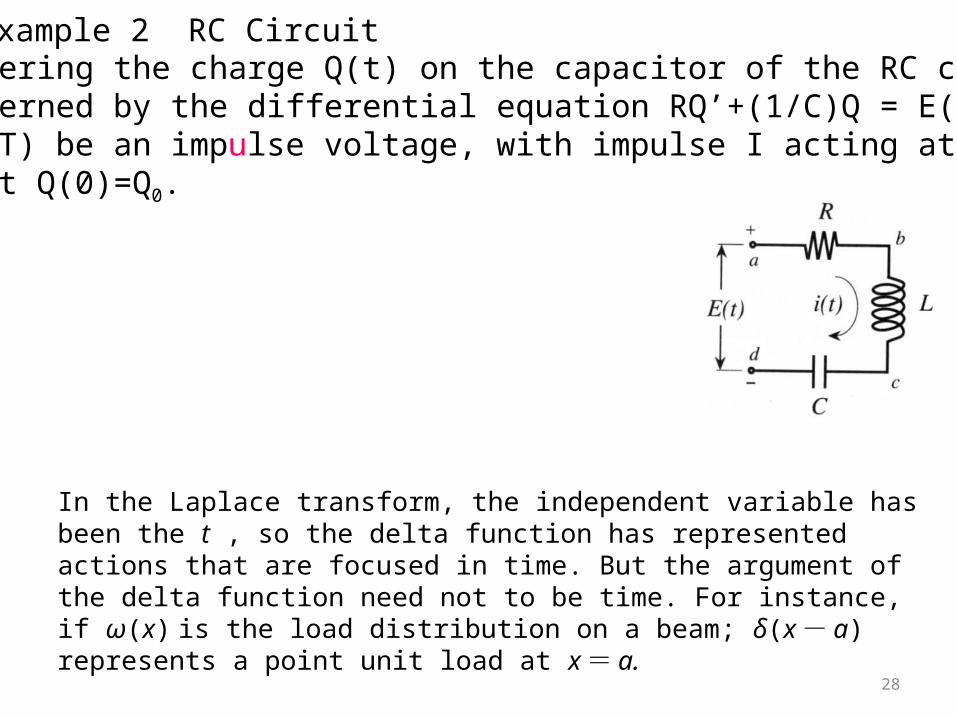
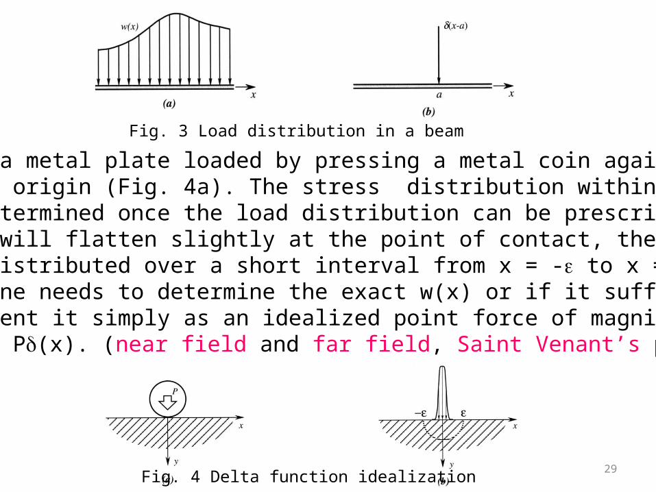
In the Laplace transform, the independent variable has been the t , so the delta function has represented actions that are focused in time. But the argument of the delta function need not to be time. For instance, if ω(x) is the load distribution on a beam; δ(x - a) represents a point unit load at x = a.
Example 2 RC CircuitConsidering the charge Q(t) on the capacitor of the RC circuit is governed by the differential equation RQ’+(1/C)Q = E(T). Let E(T) be an impulse voltage, with impulse I acting at t = T, and let Q(0)=Q0.
29
Fig. 3 Load distribution in a beam
Fig. 4 Delta function idealization
Consider a metal plate loaded by pressing a metal coin against it at the origin (Fig. 4a). The stress distribution within the plate can be determined once the load distribution can be prescribed.The coin will flatten slightly at the point of contact, the load w(x) will be distributed over a short interval from x = - to x = . Whether one needs to determine the exact w(x) or if it suffices to represent it simply as an idealized point force of magnitude P, w(x) = P(x). (near field and far field, Saint Venant’s principle)
30
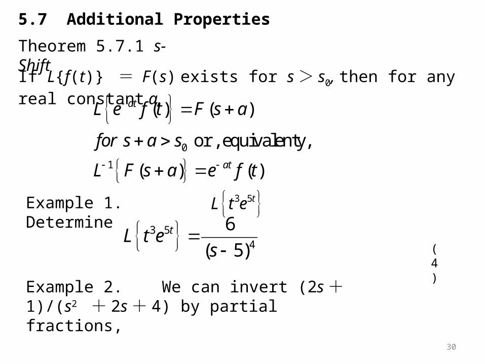
5.7 Additional Properties
Theorem 5.7.1 s-Shift
If L{f(t)} = F(s) exists for s > s0, then for any real constant a,
0
1
( ) ( )
or , equivalenty,
( ) ( )
at
at
L e f t F s a
for s a s
L F s a e f t
3 54
6
( 5)tL t e
s
3 5tL t eExample 1. Determine
(4)
Example 2. We can invert (2s + 1)/(s2 + 2s +4) by partial fractions,
31
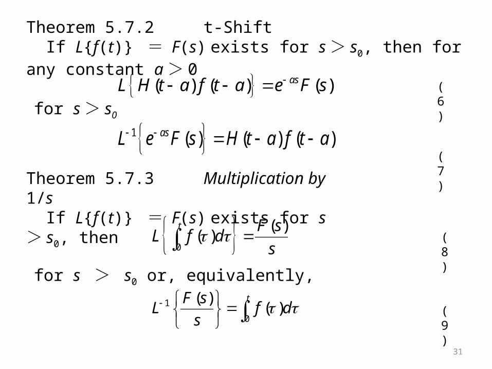
1 ( ) ( ) ( )asL e F s H t a f t a
( ) ( ) ( )asL H t a f t a e F s
Theorem 5.7.2 t-Shift If L{f(t)} = F(s) exists for s > s0, then for any constant a >0
(6)
(7)
for s > s0
1
0
( )( )
tF sL f d
s
0
( )( )
t F sL f d
s
Theorem 5.7.3 Multiplication by 1/s If L{f(t)} = F(s) exists for s > s0, then
(8)
for s > s0 or, equivalently,
(9)
32
1 ( )( )
dF sL tf t
ds
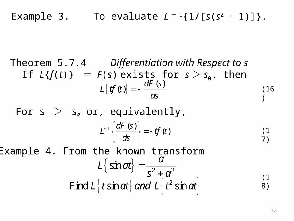
Example 3. To evaluate L - 1{1/[s(s2 + 1)]}.
( )( )
dF sL tf t
ds
Theorem 5.7.4 Differentiation with Respect to s If L{f(t)} = F(s) exists for s > s0, then
For s > s0 or, equivalently,
2 2sin
aL at
s a
Example 4. From the known transform
(18)
(17)
(16)
2Find sin sinL t at and L t at
33
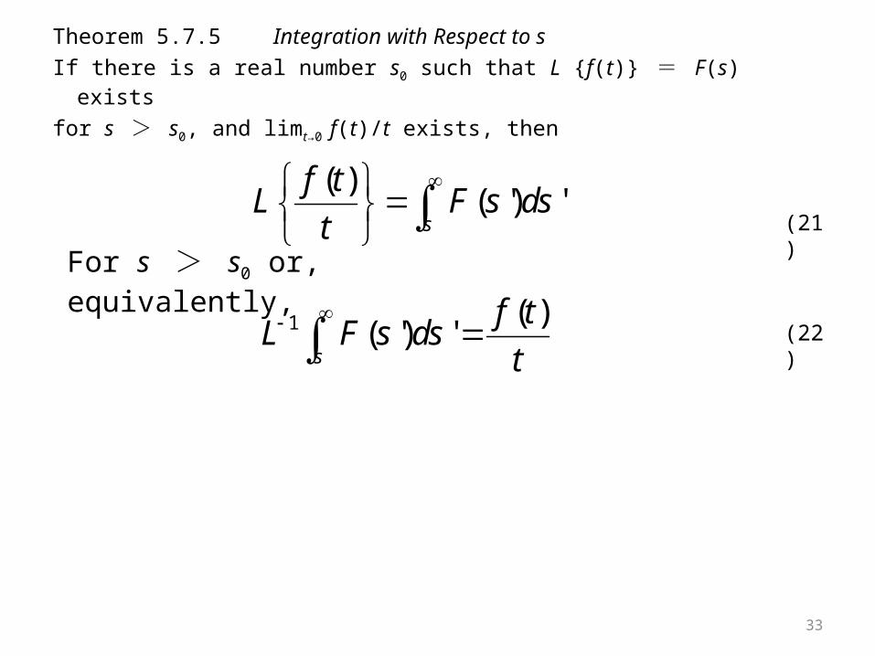
Theorem 5.7.5 Integration with Respect to s
If there is a real number s0 such that L {f(t)} = F(s) exists
for s > s0, and limt→0 f(t)/t exists, then
For s > s0 or, equivalently,
( )( ') '
s
f tL F s ds
t
(21)
(22)1 ( )( ') '
s
f tL F s ds
t
34
Theorem 5.7.6 Large s Behavior of F(s)Let f(t) be piecewise continuous on for each finite t0 and of exponential order as t → ∞. Then (i)F(s) → 0 as s → ∞,(ii)sF(s) is bounded as s → ∞.
00 t t
35
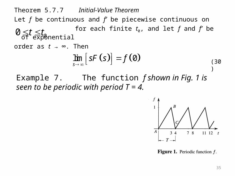
Theorem 5.7.7 Initial-Value Theorem
Let f be continuous and f’ be piecewise continuous on
for each finite t0, and let f and f’ be of exponential
order as t → ∞. Then
00 t t
Example 7. The function f shown in Fig. 1 is seen to be periodic with period T = 4.
lim 0s
sF s f
(30)
36
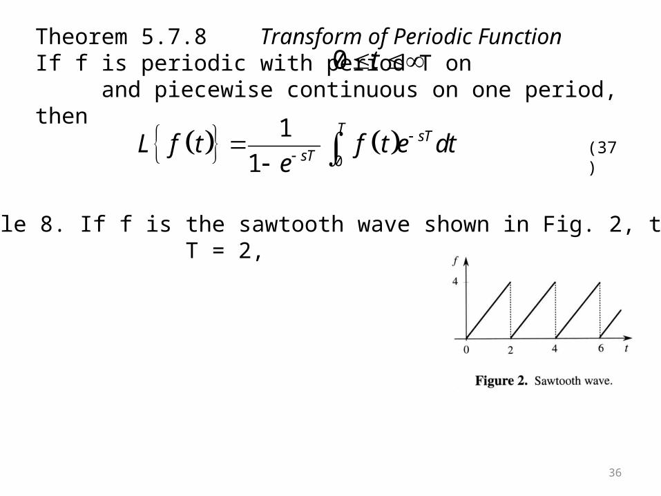
Theorem 5.7.8 Transform of Periodic FunctionIf f is periodic with period T on and piecewise continuous on one period, then
0 t
Example 8. If f is the sawtooth wave shown in Fig. 2, then T = 2,
0
1
1
T sTsT
L f t f t e dte
(37)
37
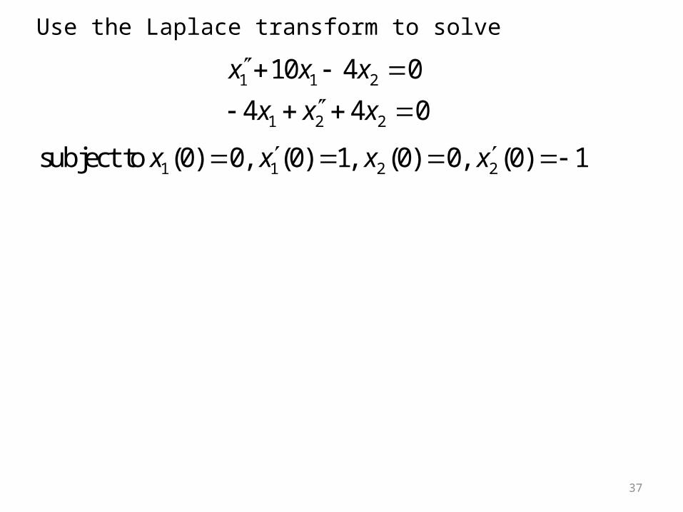
Use the Laplace transform to solve
1 1 2
1 2 2
10 4 0
4 4 0
x x x
x x x
1 1 2 2subject to (0) 0, (0) 1, (0) 0, (0) 1x x x x
38
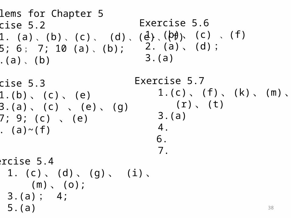
Problems for Chapter 5Exercise 5.2 1. (a) 、 (b) 、 (c) 、 (d) 、 (e) 、 (f) 5; 6 ; 7; 10 (a) 、 (b); 12.(a) 、 (b)
Exercise 5.3 1.(b) 、 (c) 、 (e) 3.(a) 、 (c) 、 (e) 、 (g) 7; 9; (c) 、 (e) 10. (a)~(f)
Exercise 5.4 1. (c) 、 (d) 、 (g) 、 (i) 、 (m) 、 (o); 3.(a) ; 4; 5.(a)
Exercise 5.6 1. (b) 、 (c) 、 (f) 2. (a) 、 (d) ; 3.(a)
Exercise 5.7 1.(c) 、 (f) 、 (k) 、 (m) 、 (r) 、 (t) 3.(a) 4. 6. 7.