1

Chapter 14 Mass-Storage Structure

2

Outline

• Disk Structure• Disk Scheduling• Disk Management• Swap-Space Management• RAID Structure• Disk Attachment• Stable-Storage Implementation• Tertiary Storage Devices

3

14.1 Disk Structure

• Disk drives are addressed as large 1-dimensional arrays of logical blocks, where the logical block is the smallest unit of transfer.

• The 1-dimensional array of logical blocks is mapped into the sectors of the disk sequentially.– Sector 0 is the first sector of the first track on the outermost cylinder.– Mapping proceeds (Cylinder, Track, Sector)

• In practice, not always possible– Defective Sectors– # of tracks per cylinders is not a constant

4

14.2 Disk Scheduling

5

Overview

• OS is responsible for using hardware efficiently– For disk drives fast access time and disk bandwidth

• Access time has two major components– Seek time is the time for the disk to move the heads to the cylinder

containing the desired sector

• Seek time seek distance

• Minimize seek time

– Rotational latency is the additional time waiting for the disk to rotate the desired sector to the disk head

• Difficult for OS

• Disk bandwidth is the total number of bytes transferred, divided by the total time between the first request for service and the completion of the last transfer

6

Overview (Cont.)

• Several algorithms exist to schedule the servicing of disk I/O requests.

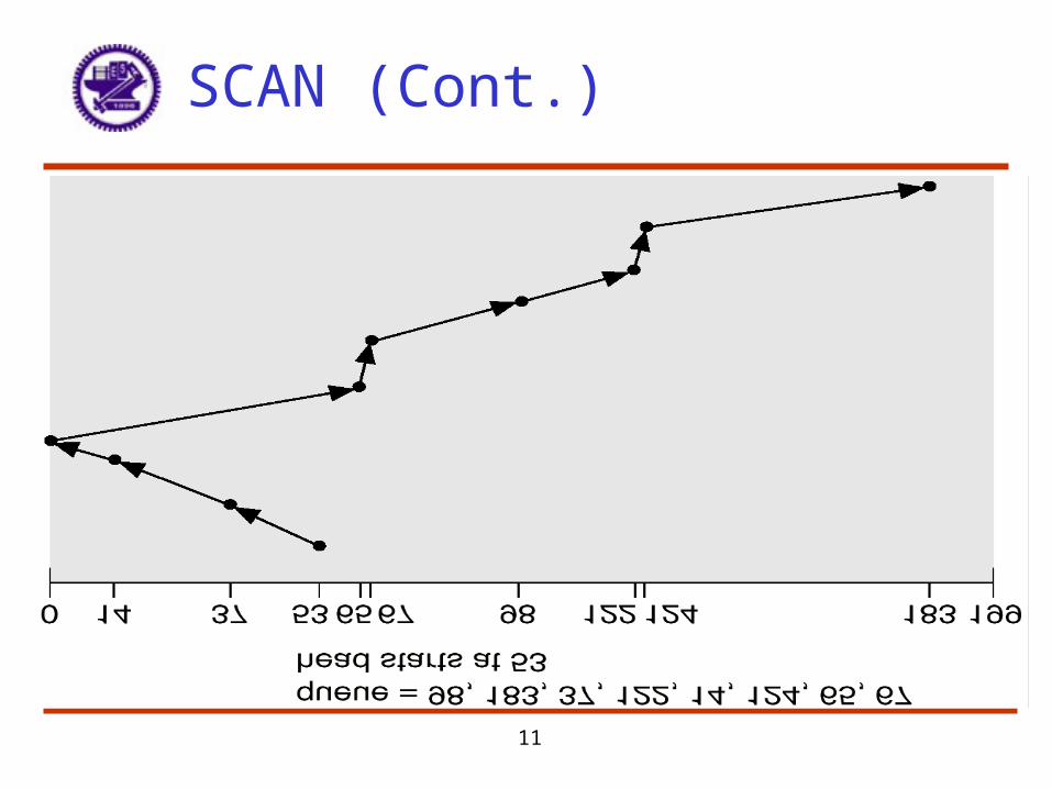
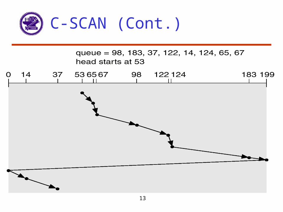
• We illustrate them with a request queue (0-199).– 98, 183, 37, 122, 14, 124, 65, 67– Head pointer 53

7

FCFS

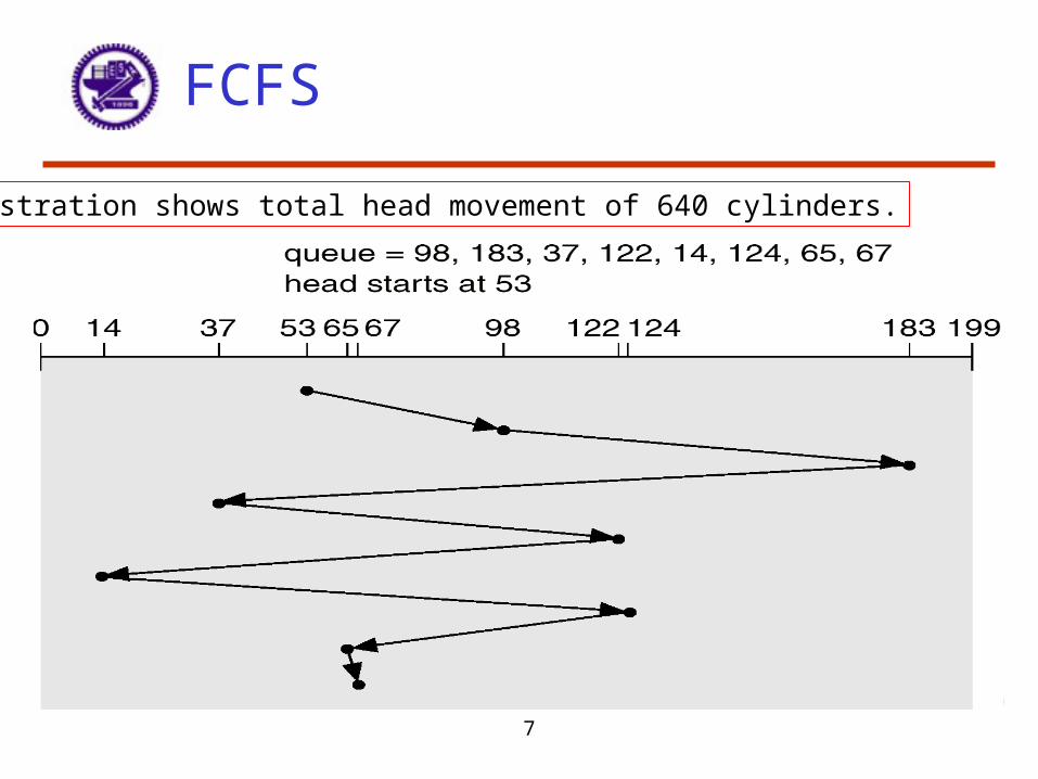
Illustration shows total head movement of 640 cylinders.

8

SSTF

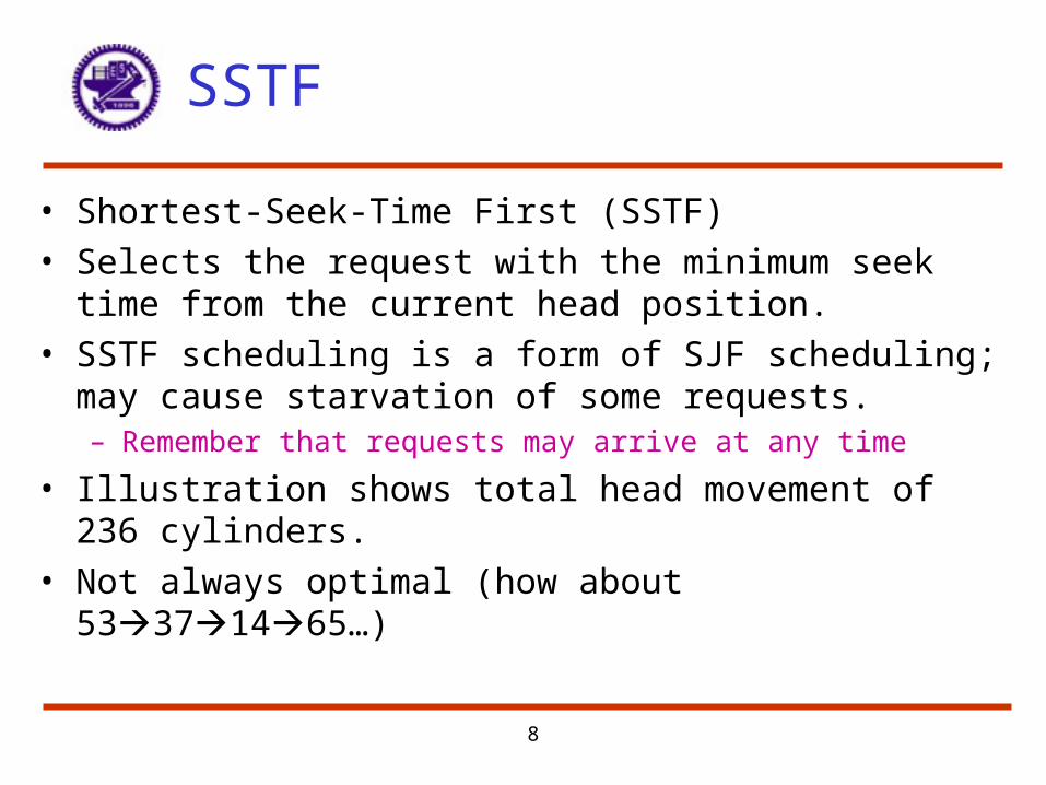
• Shortest-Seek-Time First (SSTF)• Selects the request with the minimum seek time from the

current head position.• SSTF scheduling is a form of SJF scheduling; may cause

starvation of some requests.– Remember that requests may arrive at any time

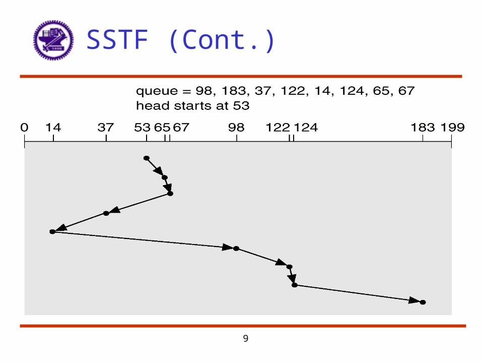
• Illustration shows total head movement of 236 cylinders.• Not always optimal (how about 53371465…)

9

SSTF (Cont.)

10

SCAN

• The disk arm starts at one end of the disk, and moves toward the other end, servicing requests until it gets to the other end of the disk, where the head movement is reversed and servicing continues.

• Sometimes called the elevator algorithm.• Illustration shows total head movement of 208 cylinders.

11

SCAN (Cont.)

12

C-SCAN

• Provides a more uniform wait time than SCAN.• The head moves from one end of the disk to the other,

servicing requests as it goes. When it reaches the other end, however, it immediately returns to the beginning of the disk, without servicing any requests on the return trip.

• Treats the cylinders as a circular list that wraps around from the last cylinder to the first one.

13

C-SCAN (Cont.)

14

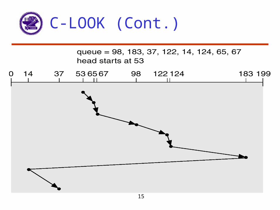
C-LOOK

• Version of C-SCAN• Arm only goes as far as the last request in each direction,

then reverses direction immediately, without first going all the way to the end of the disk.

15

C-LOOK (Cont.)

16

Selecting a Disk-Scheduling Algorithm

• SSTF is common and has a natural appeal• SCAN and C-SCAN perform better for systems that place a heavy load

on the disk• Performance relies on the number and types of requests• Requests for disk service can be influenced by the file-allocation method

(Contiguous? Linked? Indexed?)• The disk-scheduling algorithm should be written as a separate module

of the operating system, allowing it to be replaced with a different algorithm if necessary

• Either SSTF or LOOK is a reasonable choice for the default algorithm• Scheduled by OS? Scheduled by disk controller?

17

14.3 Disk Management

18

Disk Formatting

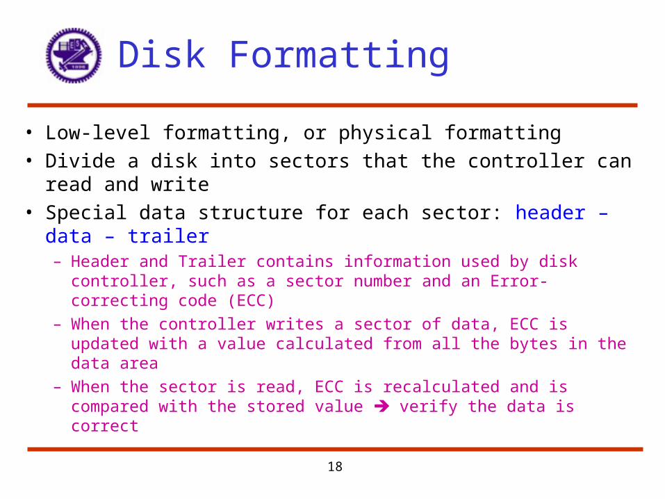
• Low-level formatting, or physical formatting• Divide a disk into sectors that the controller can read and

write• Special data structure for each sector: header – data –

trailer– Header and Trailer contains information used by disk controller, such

as a sector number and an Error-correcting code (ECC)– When the controller writes a sector of data, ECC is updated with a

value calculated from all the bytes in the data area– When the sector is read, ECC is recalculated and is compared with

the stored value verify the data is correct

19

Disk Partition

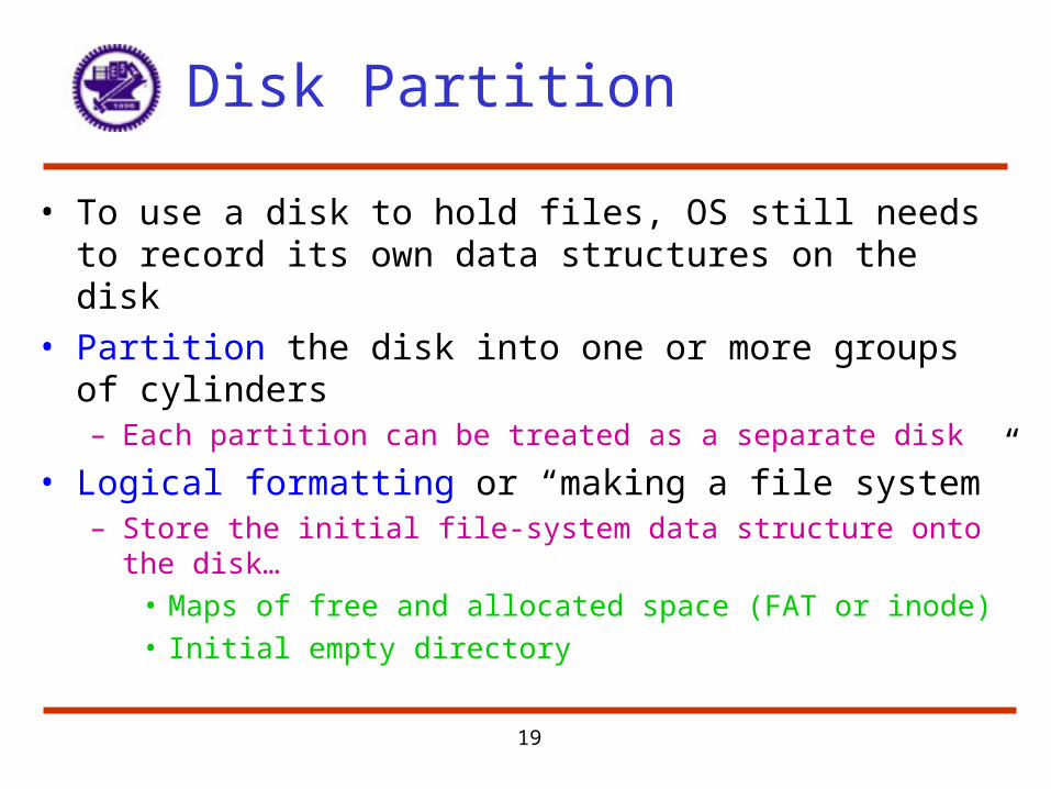
• To use a disk to hold files, OS still needs to record its own data structures on the disk

• Partition the disk into one or more groups of cylinders– Each partition can be treated as a separate disk

• Logical formatting or “making a file system”– Store the initial file-system data structure onto the disk…

• Maps of free and allocated space (FAT or inode)• Initial empty directory

20

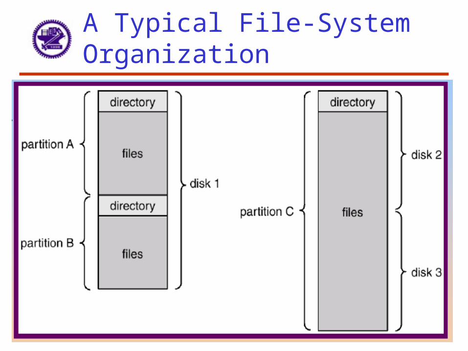
A Typical File-System Organization

21

Raw Disk

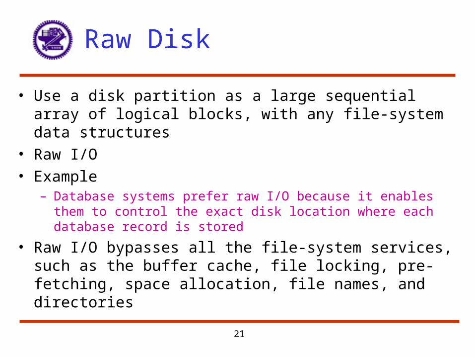
• Use a disk partition as a large sequential array of logical blocks, with any file-system data structures

• Raw I/O• Example

– Database systems prefer raw I/O because it enables them to control the exact disk location where each database record is stored

• Raw I/O bypasses all the file-system services, such as the buffer cache, file locking, pre-fetching, space allocation, file names, and directories

22

Boot Block

• Boot block initializes system– Initialize CPU registers, device controllers, main memory– Start OS

• A tiny bootstrap loader is stored in boot ROM– Bring a full bootstrap program from disk

• Full bootstrap program is stored in boot blocks (fixed location)

• The boot ROM instructs the disk controller to read the boot blocks into memory, and then start executing the code to load the entire OS

23

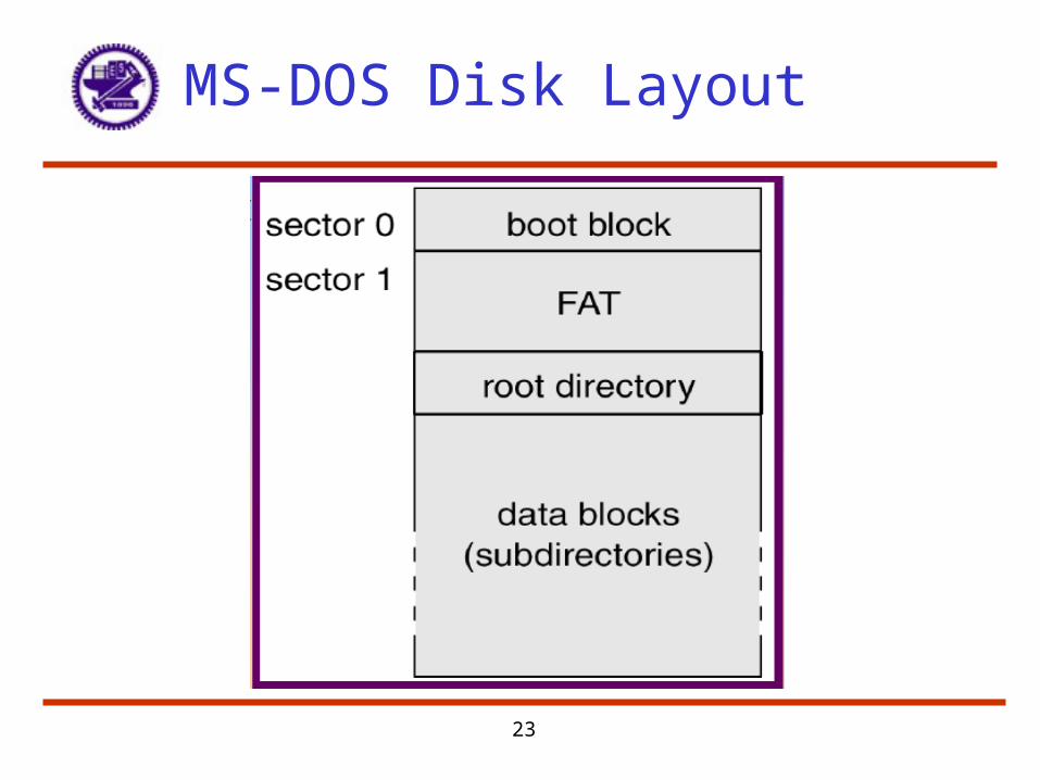
MS-DOS Disk Layout

24

Bad Blocks

• IDE– MS-DOS format : write a special value into the corresponding FAT

entry for bad blocks– MS-DOS chkdsk : search and lock bad blocks

25

Bad Blocks – SCSI (Cont.)

• Controller maintains a list of bad blocks on the disk• Low-level formatting spare sectors (OS don’t know)• Controller replaces each bad sector logically with one of the

spare sectors (sector sparing, or forwarding)– Invalidate optimization by OS’s disk scheduling– Each cylinder has a few spare sectors

26

Bad Blocks – SCSI (Cont.)

• Typical bad-sector transaction– OS tries to read logical block 87– Controller calculates ECC and finds that it is bad. Report to OS– Reboot next time, a special command is run to tell the controller to

replace the bad sector with a spare.– Whenever the system requests block 87, it is translated into the

replacement sector’s address by the controller

• Sector slipping:– Ex. 17 defective, spare follows sector 202

• Spare 202 201 … 18 17

27

14.4 Swap-Space Management

28

Swap-Space Use

• Swap-space — Virtual memory uses disk space as an extension of main memory

• Main goal for the design and implementation of swap space is to provide the best throughput for VM system

• Swap-space use– Swapping – use swap space to hold entire process image– Paging – simple store pages that have been pushed out of memory

• Some OS may support multiple swap-space– Put on separate disks to balance the load

• Better to overestimate than underestimate– If out of swap-space, some processes must be aborted or system

crashed

29

Swap-Space Location

• Swap-space: In a separate disk partition or in a normal file system (in UNIX, mkfile and swapadd (or fstab, vfstab))– Convenience of allocation and management in the file system, and

the performance of swapping in raw partitions

• Swap-space in a file-system – simply a large file– Navigating the directory structure and the disk-allocation data

structure takes time and potentially extra disk accesses– External fragmentation can greatly increase swapping times by

forcing multiple seeks during reading or writing of a process image– Improve by caching in main memory and contiguous allocation

• The cost of traversing FS data structure still remains

30

Swap-Space Location (Cont.)

• Swap-space in a separate partition– Create a fixed amount of swap space during disk partitioning– Raw partition– A separate swap-space storage manager is used to allocate and de-

allocate blocks– Use algorithms optimized for speed, rather than storage efficiency– Internal fragment may increase

• Some OS supports both

31

Swap-space Management (Example)

• 4.3BSD allocates swap space when process starts; holds text segment (the program) and data segment.– Kernel uses swap maps to track swap-space use

• Solaris 1: text-segment pages (clean pages) are brought in from the file system and are thrown away if selected for paged out (more efficient)

• Solaris 2: allocates swap space only when a page is forced out of physical memory, not when the virtual memory page is first created.

32

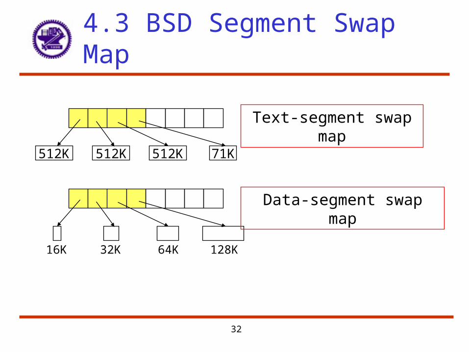
4.3 BSD Segment Swap Map

512K 512K 512K 71K

Text-segment swap map

Data-segment swap map

16K 32K 64K 128K

33

14.5 RAID Structure

34

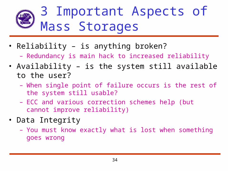
3 Important Aspects of Mass Storages

• Reliability – is anything broken?– Redundancy is main hack to increased reliability

• Availability – is the system still available to the user?– When single point of failure occurs is the rest of the system still

usable?– ECC and various correction schemes help (but cannot improve

reliability)

• Data Integrity– You must know exactly what is lost when something goes wrong

35

Disk Arrays

• Multiple arms improve throughput, but not necessarily improve latency

• Striping– Spreading data over multiple disks

• Reliability– General metric is N devices have 1/N reliability

• Rule of thumb: MTTF of a disk is about 5 years– Hence need to add redundant disks to compensate

• MTTR ::= mean time to repair (or replace) (hours for disks)• If MTTR is small then the array’s MTTF can be pushed out

significantly with a fairly small redundancy factor

36

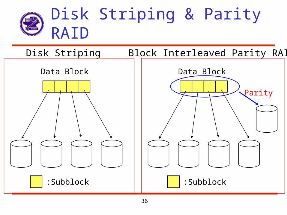
Disk Striping & Parity RAID

Data Block

:Subblock

Disk Striping

Data Block

:Subblock

Block Interleaved Parity RAID

Parity

37

Data Striping

• Bit-level striping: split the bit of each bytes across multiple disks– No. of disks can be a multiple of 8 or divides 8

• Block-level striping: blocks of a file are striped across multiple disks; with n disks, block i goes to disk (i mod n)+1

• Every disk participates in every access– Number of I/O per second is the same as a single disk– Number of data per second is improved

• Provide high data-transfer rates, but not improve reliability

38

Redundant Arrays of Disks

• Files are "striped" across multiple disks• Availability is improved by adding redundant disks

– If a single disk fails, the lost information can be reconstructed from redundant information

– Capacity penalty to store redundant information– Bandwidth penalty to update

• RAID– Redundant Arrays of Inexpensive Disks– Redundant Arrays of Independent Disks

• Hot Spare and Hot Swap

39

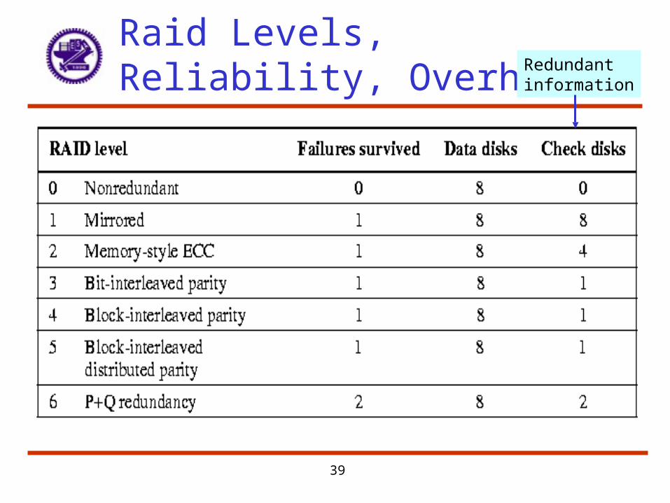
Raid Levels, Reliability, Overhead Redundant

information

40

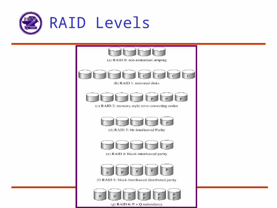
RAID Levels

41

RAID Levels 0 - 1

• RAID 0 – No redundancy (Just block striping)– Cheap but unable to withstand even a single failure

• RAID 1 – Mirroring – Each disk is fully duplicated onto its "shadow“– Files written to both, if one fails flag it and get data from the mirror– Reads may be optimized – use the disk delivering the data first– Bandwidth sacrifice on write: Logical write = two physical writes– Most expensive solution: 100% capacity overhead– Targeted for high I/O rate , high availability environments

• RAID 0+1 – stripe first, then mirror the stripe• RAID 1+0 – mirror first, then stripe the mirror

42

RAID Levels 2 & 3

• RAID 2 – Memory style ECC– Cuts down number of additional disks

– Actual number of redundant disks will depend on correction model

– RAID 2 is not used in practice

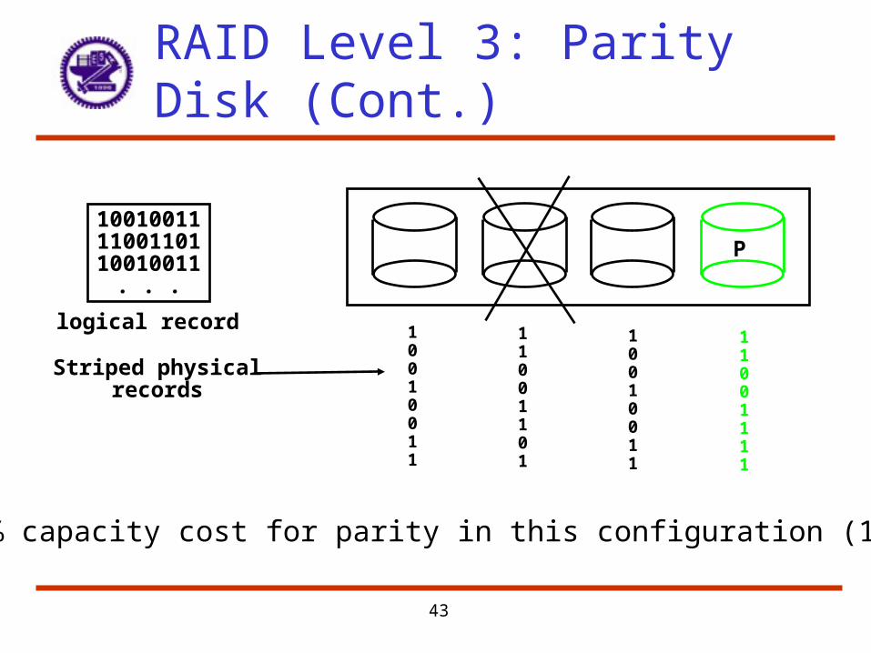
• RAID 3 – Bit-interleaved parity– Reduce the cost of higher availability to 1/N (N = # of disks)

– Use one additional redundant disk to hold parity information

– Bit interleaving allows corrupted data to be reconstructed

– Interesting trade off between increased time to recover from a failure and cost reduction due to decreased redundancy

– Parity = sum of all relative disk blocks (module 2)

• Hence all disks must be accessed on a write – potential bottleneck

– Targeted for high bandwidth applications: Scientific, Image Processing

43

P100100111100110110010011

. . .

logical record 10010011

11001101

10010011

11001111

Striped physicalrecords

25% capacity cost for parity in this configuration (1/N)

RAID Level 3: Parity Disk (Cont.)

44

RAID Levels 4 & 5 & 6

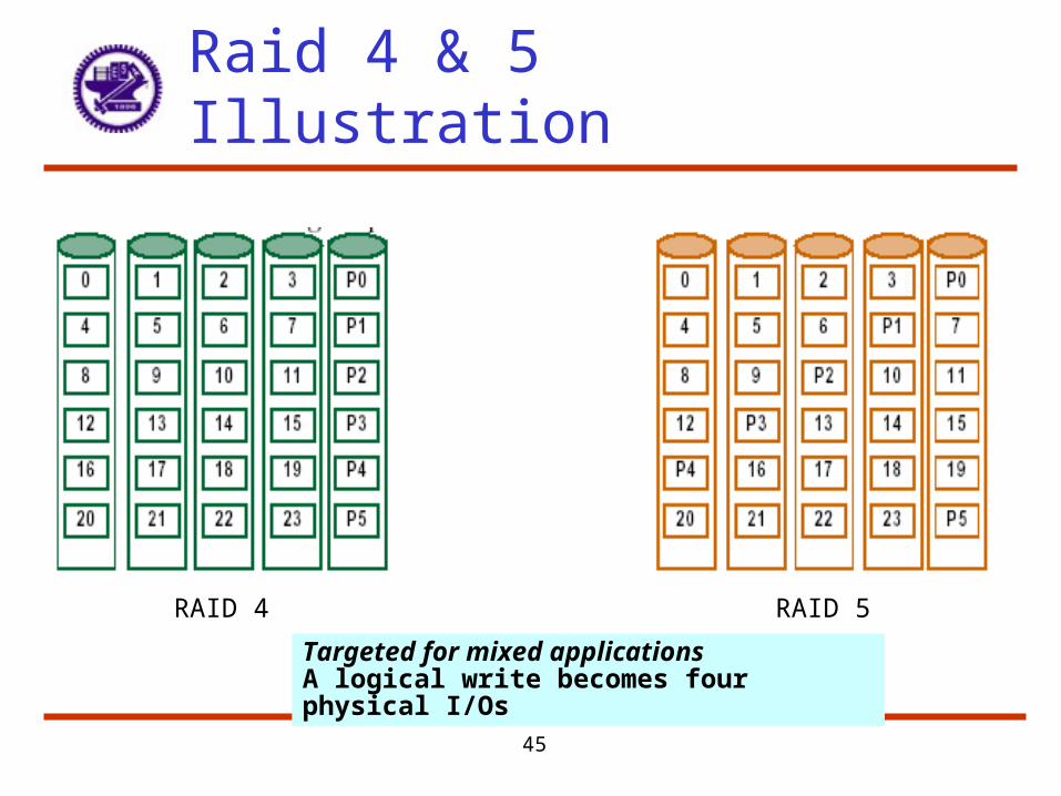
• RAID 4 – Block interleaved parity– Similar idea as RAID 3 but sum is on a per block basis– Hence only the parity disk and the target disk need be accessed– Problem still with concurrent writes since parity disk bottlenecks

• RAID 5 – Block interleaved distributed parity– Parity blocks are interleaved and distributed on all disks– Hence parity blocks no longer reside on same disk– Probability of write collisions to a single drive are reduced– Hence higher performance in the consecutive write situation

• RAID 6– Similar to RAID 5, but stores extra redundant information to guard

against multiple disk failures

45

Raid 4 & 5 Illustration

RAID 4 RAID 5

Targeted for mixed applicationsA logical write becomes four physical I/Os

46

14.6 Disk Attachment

47

Disk Attachment

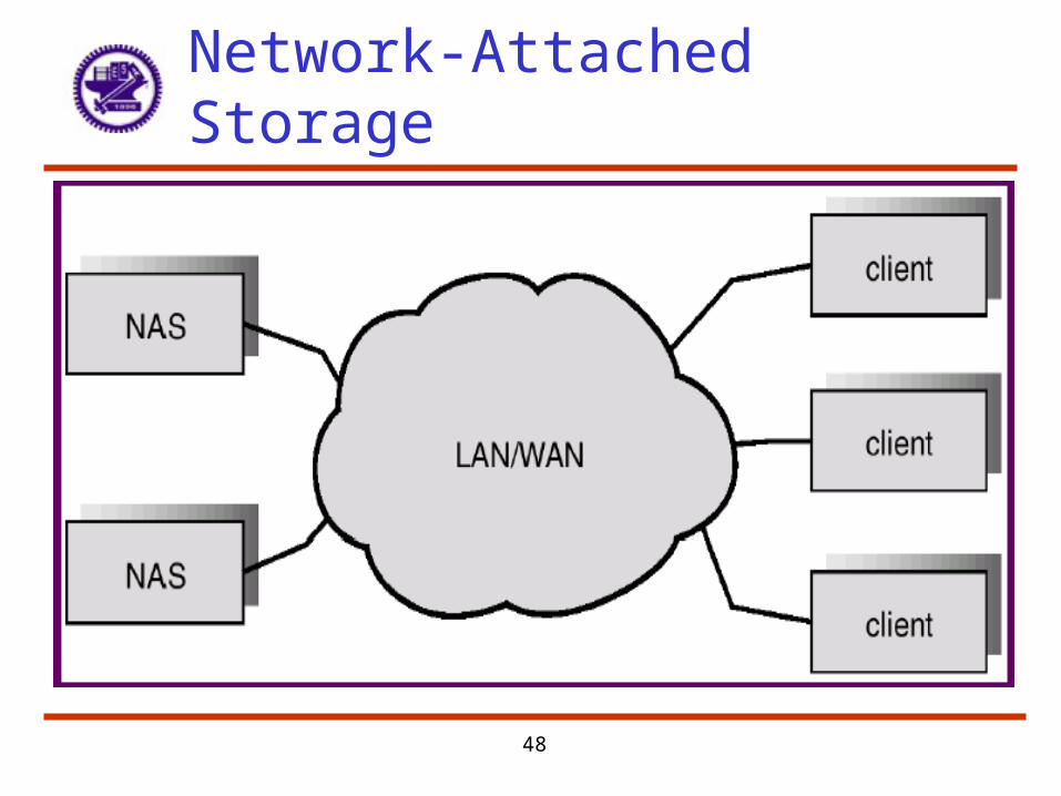
• Disks may be attached one of two ways:• Host attached via an I/O port• Network attached via a network connection• Network-attached storage – implemented as a RAID array

with software that implements RPC interface for NFS (UNIX machines) or CIFS (Windows machines)

• Storage-area network – a private network (using storage protocols rather than network protocols) among servers and storage units, separate from LAN or WAN connecting clients and servers

48

Network-Attached Storage

49

Storage Area Network

50

14.7 Stable-Storage Implementation

51

Overview

• Information residing in stable storage is never lost• To implement stable storage:

– Replicate information on more than one nonvolatile storage media with independent failure modes

– Coordinate the writing of updates in a way that guarantees that a failure during an update will not leave all the copies in a damaged state, to ensure that we can recover the stable data after any failure during data transfer or recovery

52

Disk Write Result

• Successful Completion• Partial Failure: failure occurred in the midst of transfer, so

some of the sectors were written with the new data, and the sector being written during the failure may have been corrupted

• Total Failure: failure occurred before the disk write started, so the previous data value on the disk remain intact

53

Recoverable Write

• System must maintain (at least) 2 physical blocks for each logical block, for detecting and recovering from failure

• Recoverable write– Write the information onto the first physical block– When the first write completes successfully, write the same

information onto the second physical block– Declare the operation complete only after the second write

completes successfully

54

Failure Detection and Recovery

• Each pair of physical blocks is examined• If both are the same and no detectable error exists OK• If one contains a detectable error, then we replace its

contents with the value of the other block• If both contain no detectable error, but they differ in content,

then we replace the content of the first block with the value of the second

• Ensure that a write to stable storage either succeeds completely or results in no change

55

14.8 Tertiary-Storage Structure

56

Tertiary Storage Devices

• Low cost is the defining characteristic of tertiary storage.• Generally, tertiary storage is built using removable media• Common examples of removable media are floppy disks

and CD-ROMs; other types are available.

57

Removable Disks

• Floppy disk — thin flexible disk coated with magnetic material, enclosed in a protective plastic case.– Most floppies hold about 1 MB; similar technology is used for

removable disks that hold more than 1 GB.– Removable magnetic disks can be nearly as fast as hard disks, but

they are at a greater risk of damage from exposure.

58

Removable Disks (Cont.)

• A magneto-optic disk records data on a rigid platter coated with magnetic material.– Laser heat is used to amplify a large, weak magnetic field to record a

bit.– Laser light is also used to read data (Kerr effect).– The magneto-optic head flies much farther from the disk surface

than a magnetic disk head, and the magnetic material is covered with a protective layer of plastic or glass; resistant to head crashes.

• Optical disks do not use magnetism; they employ special materials that are altered by laser light.

59

WORM Disks

• The data on read-write disks can be modified over and over.• WORM (“Write Once, Read Many Times”) disks can be

written only once.• Thin aluminum film sandwiched between two glass or plastic

platters.• To write a bit, the drive uses a laser light to burn a small

hole through the aluminum; information can be destroyed by not altered.

• Very durable and reliable.• Read Only disks, such ad CD-ROM and DVD, com from the

factory with the data pre-recorded.

60

Tapes

• Compared to a disk, a tape is less expensive and holds more data, but random access is much slower.

• Tape is an economical medium for purposes that do not require fast random access, e.g., backup copies of disk data, holding huge volumes of data.

• Large tape installations typically use robotic tape changers that move tapes between tape drives and storage slots in a tape library.– stacker – library that holds a few tapes

– silo – library that holds thousands of tapes

• A disk-resident file can be archived to tape for low cost storage; the computer can stage it back into disk storage for active use.

61

Operating System Issues

• Major OS jobs are to manage physical devices and to present a virtual machine abstraction to applications

• For hard disks, the OS provides two abstraction:– Raw device – an array of data blocks.– File system – the OS queues and schedules the interleaved

requests from several applications.

62

Application Interface

• Most OSs handle removable disks almost exactly like fixed disks — a new cartridge is formatted and an empty file system is generated on the disk.

• Tapes are presented as a raw storage medium, i.e., and application does not not open a file on the tape, it opens the whole tape drive as a raw device.– Usually the tape drive is reserved for the exclusive use of that

application.– Since the OS does not provide file system services, the application

must decide how to use the array of tape blocks.– Since every application makes up its own rules for how to organize a

tape, a tape full of data can generally only be used by the program that created it.

63

Tape Drives

• The basic operations for a tape drive differ from those of a disk drive.

• locate positions the tape to a specific logical block, not an entire track (corresponds to seek).

• The read position operation returns the logical block number where the tape head is.

• The space operation enables relative motion.• Tape drives are “append-only” devices; updating a block in

the middle of the tape also effectively erases everything beyond that block.

• An EOT mark is placed after a block that is written.

64

File Naming

• The issue of naming files on removable media is especially difficult when we want to write data on a removable cartridge on one computer, and then use the cartridge in another computer.

• Contemporary OSs generally leave the name space problem unsolved for removable media, and depend on applications and users to figure out how to access and interpret the data.

• Some kinds of removable media (e.g., CDs) are so well standardized that all computers use them the same way.

65

Hierarchical Storage Management (HSM)

• A hierarchical storage system extends the storage hierarchy beyond primary memory and secondary storage to incorporate tertiary storage — usually implemented as a jukebox of tapes or removable disks.

• Usually incorporate tertiary storage by extending the file system.– Small and frequently used files remain on disk.– Large, old, inactive files are archived to the jukebox.

• HSM is usually found in supercomputing centers and other large installations that have enormous volumes of data.

66

Speed

• Two aspects of speed in tertiary storage are bandwidth and latency.

• Bandwidth is measured in bytes per second.– Sustained bandwidth – average data rate during a large transfer; #

of bytes/transfer time.Data rate when the data stream is actually flowing.

– Effective bandwidth – average over the entire I/O time, including seek or locate, and cartridge switching. Drive’s overall data rate.

67

Speed (Cont.)

• Access latency – amount of time needed to locate data.– Access time for a disk – move the arm to the selected cylinder and

wait for the rotational latency; < 35 milliseconds.– Access on tape requires winding the tape reels until the selected

block reaches the tape head; tens or hundreds of seconds.– Generally say that random access within a tape cartridge is about a

thousand times slower than random access on disk.

• The low cost of tertiary storage is a result of having many cheap cartridges share a few expensive drives.

• A removable library is best devoted to the storage of infrequently used data, because the library can only satisfy a relatively small number of I/O requests per hour.

68

Reliability

• A fixed disk drive is likely to be more reliable than a removable disk or tape drive.

• An optical cartridge is likely to be more reliable than a magnetic disk or tape.

• A head crash in a fixed hard disk generally destroys the data, whereas the failure of a tape drive or optical disk drive often leaves the data cartridge unharmed.

69

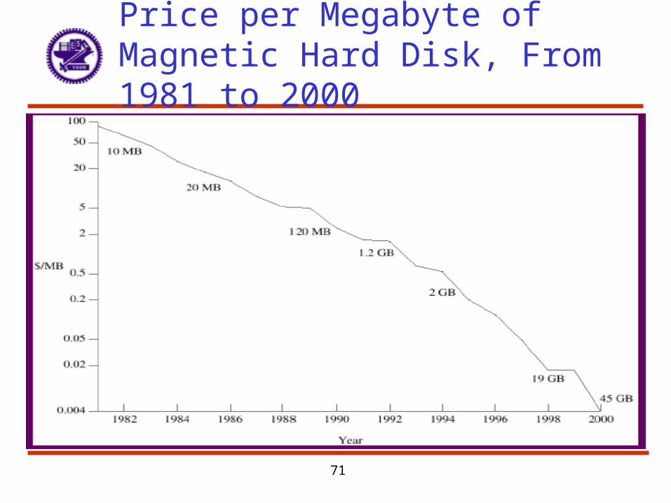
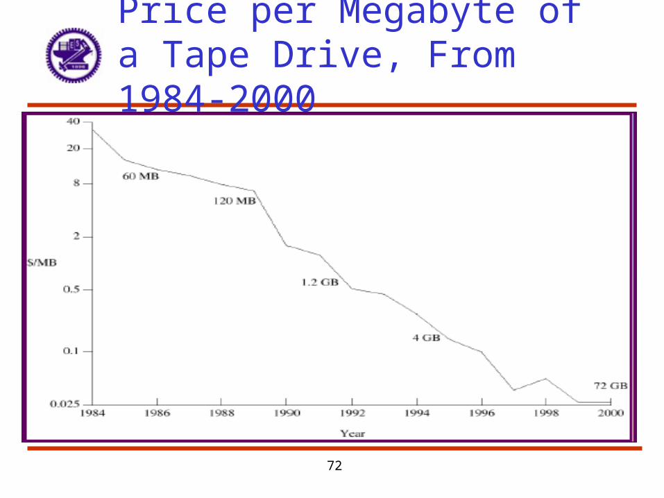
Cost

• Main memory is much more expensive than disk storage• The cost per megabyte of hard disk storage is competitive

with magnetic tape if only one tape is used per drive.• The cheapest tape drives and the cheapest disk drives have

had about the same storage capacity over the years.• Tertiary storage gives a cost savings only when the number

of cartridges is considerably larger than the number of drives.

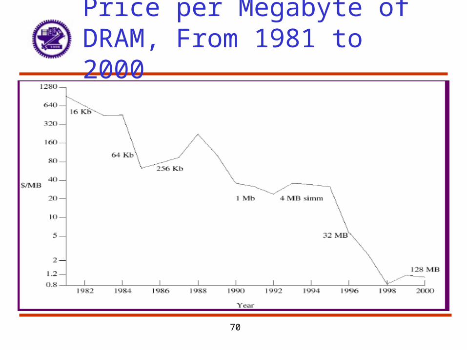
70

Price per Megabyte of DRAM, From 1981 to 2000

71

Price per Megabyte of Magnetic Hard Disk, From 1981 to 2000

72

Price per Megabyte of a Tape Drive, From 1984-2000