Embed Size (px)
Citation preview

1
Activated Sludge Model 2d calibration with full-scale WWTP data: comparing 1
model parameter identifiability with influent and operational uncertainty. 2
3
Vinicius Cunha Machado, Javier Lafuente, Juan Antonio Baeza* 4
5
Department of Chemical Engineering, Universitat Autònoma de Barcelona, ETSE, 6
08193 Bellaterra (Barcelona), Spain. Phone: +34935811587. FAX: +34935812013. 7
E-mails: [email protected], [email protected], 8
10
*Corresponding Author 11
12

2
Abstract 13
The present work developed a model for the description of a full-scale WWTP 14
(Manresa, Catalonia, Spain) for further plant upgrades based on the systematic 15
parameter calibration of the ASM2d model using a methodology based on the Fisher 16
Information Matrix (FIM). The influent was characterized for the application of the 17
ASM2d and the confidence interval of the calibrated parameters was also assessed. No 18
expert knowledge was necessary for model calibration and a huge available plant 19
database was converted into more useful information. The effect of the influent and 20
operating variables on the model fit was also studied using these variables as calibrating 21
parameters and keeping the ASM2d kinetic and stoichiometric parameters, which 22
traditionally are the calibration parameters, at their default values. Such an “inversion” 23
of the traditional way of model fitting allowed evaluating the sensitivity of the main 24
model outputs regarding to the influent and to the operating variables changes. This new 25
approach is able to evaluate the capacity of the operational variables used by the WWTP 26
feedback control loops to overcome external disturbances in the influent and 27
kinetic/stoichiometric model parameters uncertainties. In addition, the study of the 28
influence of operating variables on the model outputs provides useful information to 29
select input and output variables in decentralized control structures. 30
31
Keywords: ASM2d, EBPR, FIM, full-scale WWTP, calibration, influent 32
characterization, modelling. 33
34

3
35
Nomenclature 36
A2/O Anaerobic, Anoxic and Aerobic (WWTP configuration) 37
ASM Activated Sludge Models 38
BOD5 Biological Oxygen Demand (5 days) 39
CCF Calibration Cost Function 40
COD Chemical Oxygen Demand 41
DO Dissolved Oxygen 42
EBPR Enhanced Biological Phosphorus Removal 43
FIM Fisher Information Matrix 44
GAO Glycogen Accumulating Organisms 45
IWA International Water Association 46
PAO Phosphorus Accumulating Organisms 47
PCCF Preliminary Calibration Cost Function 48
PID Proportional-Integral-Derivative controller 49
SRT Sludge Retention Time 50
TKN Total Kjeldahl Nitrogen 51
TN Total Nitrogen 52
TSS Total Suspended Solids 53
VCF Validation Cost Function 54
WWTP Wastewater Treatment Plant 55
WERF Water Environment Research Foundation 56
57

4
1. Introduction 58
Modelling wastewater treatment plants (WWTP) is the fundamental stone to improve 59
WWTP performance through identifying bottlenecks and proposing modifications of 60
existent plants or to design a completely new one. Besides the experimental knowledge, 61
mathematical models are a set of tools for predicting plant behaviour under different 62
conditions from the ordinary outlook of the WWTP or under unexpected operational 63
scenarios [1]. The models are also useful for changing process concepts and developing 64
new plant configurations [2]. The operation of WWTPs is based on the behaviour of 65
different microorganisms, which are responsible for biological nutrient (nitrogen and 66
phosphorus) and organic matter (carbon) removal. Such processes are well described by 67
the IWA models ASM1, ASM2, ASM2d and ASM3, even though other models have 68
been used and accepted in practical and scientific media as the TUD-P model [3–5] or 69
the ASM3 EAWAG Bio-P [6]. ASM2d model is being used in many researches 70
concerning WWTP due to including the most important biological processes of ordinary 71
heterotrophic biomass, heterotrophic PAO biomass and nitrifiers. Ferrer et al. [7] used 72
this model to fit full-scale WWTP data and then to evaluate different configurations for 73
improving nutrient removal. Ingildsen et al. [8] calibrated the ASM2d model for the 74
Avedøre WWTP (Denmark) to support a control strategy for maintaining the enhanced 75
biological phosphorus removal (EBPR) process activated for long periods. Xie et al. [9] 76
also used ASM2d to simulate and optimize a full-scale Carrousel WWTP. García-Usach 77
et al. [10] or Machado et al. [11] successfully used ASM2d for describing EBPR 78
process at pilot scale. 79
WWTP models are also useful for studying and proposing several control strategies in 80
order to guarantee the effluent quality with or without external disturbances (storm 81
events, peaks of pollutants in the influent…). The effluent quality is the main goal of the 82

5
control structures, where ammonium, nitrate and phosphorus are the main pollutants 83
that should be kept at lower values to avoid the eutrophication effect. Nevertheless, 84
dissolved oxygen (DO) and the sludge residence time (SRT) are the inventory variables 85
that should be controlled first [12]. To control ammonium concentration, a cascade 86
controller which calculates the DO setpoint in the aerobic basin using the error between 87
the desired ammonium concentration and the real measurement in the effluent is 88
designed [13]. An ammonium feedback-feedforward controller also could be 89
implemented if the ammonium influent load is estimated or measured [14]. Nitrate 90
removal is accomplished by the denitrification processes which depend on the readily 91
organic matter available in an anoxic zone and the nitrate concentration. Two ways of 92
controlling the nitrate concentration at the effluent is adding external carbon source and 93
changing the nitrate recycle from the aerobic basin to the anoxic one in most of WWTP 94
[15, 16]. It is worth noticing that the measured and the manipulated variables also have 95
uncertainties, like recycling flow measurements and dissolved oxygen concentrations. 96
All the abovementioned control applications using WWTP models should be preceded 97
by a correlation analysis of the available manipulated variables not to add internal 98
disturbances to control the effluent quality. 99
Despite all the cited models are essential tools for improving many aspects of the 100
wastewater treatment, they are structured on kinetic and stoichiometric parameters that 101
should be identified for better accuracy. Besides, their state variables are not exactly the 102
same as the information obtained from laboratory analysis periodically performed in the 103
WWTP. Therefore, it is necessary, first, to convert some daily plant measurements of 104
the influent into model states and, second, to calibrate parameters using plant data and 105
lab assays (batch tests with the plant biomass). In the literature it is possible to find a 106
methodology to accomplish the first task before mentioned [17], although the influent 107

6
identifiability linked to its variability has not received much attention. The parameter 108
calibration could be performed using protocols reported in the literature [18, 19] as the 109
protocols developed by STOWA [20], BIOMATH [21], WERF [22], HSG [23] or 110
Mannina et al. [24, 25]. All these protocols are good at posing well the goals of the 111
calibration, systematically treat the plant data gathered and have a validation step with 112
different data from those used to calibrate the model. On the other hand, only 113
BIOMATH, WERF or Mannina et al. protocols pay attention to the parameter subset 114
selection to maximize the information mined from the plant data. Machado et al. [11], 115
developed an alternative calibration methodology, called the “seeds methodology”, 116
using criteria derived from the Fisher Information Matrix (FIM) to avoid overfitting. 117
Although the hydraulics modelling and a detailed biomass characterization are not 118
emphasized in this last method as in the HSG and BIOMATH protocols, respectively, 119
the usage of a large amount of available plant data combined with a systematic 120
procedure to find the most identifiable parameters subset, without testing all the 121
possible parameters combinations, are the strengths of the “seeds methodology”. 122
Unfortunately, the performance of all the abovementioned protocols is affected by 123
uncertainties from different sources during the modelling task. Refsgaard et al. [26] 124
pointed out that several error sources affect the quality of model simulation results: (i) 125
context and framing; (ii) input uncertainty; (iii) model structure uncertainty; (iv) 126
parameter uncertainty and (v) model technical uncertainty. Sin et al. [27] deepened in 127
the uncertainty analysis, concluding that both biokinetic/stoichiometric/influent 128
fractionation related parameters as well as hydraulics/mass transfer related parameters 129
induced significant uncertainty in the predicted performance of WWTP. Moreover, 130
Cierkens et al. [28] studied the effect of the influent data frequency on the calibration 131
quality and output uncertainty of the WWTP model fit. 132

7
Uncertainty assessment of kinetic and stoichiometric model parameters of ASM1 and 133
ASM2 has been applied for full-scale WWTP as in Mannina et al. [29], who evaluated 134
the model reliability identifying the crucial aspects where higher uncertainty rely and 135
more efforts should be provided in terms of both data gathering and modelling practises. 136
The uncertainty associated to operation and design parameters of WWTP have also been 137
studied [30] showing that they are the most sensitive parameters for some 138
benchmarking studies. Finally, Belia et al. [31] pointed out that identifying and 139
quantifying the uncertainties involved in a new design or plant upgrade becomes crucial 140
because WWTP are required to operate with increased energy efficiency and close to 141
their limits. They also note the need for the development of a protocol to include 142
uncertainty evaluations in model-based design and optimisation projects. 143
To consider some kind of those commented uncertainties on the modelling task and 144
concentrating effort at the calibration step, the present work developed an AS model for 145
the Manresa WWTP (Manresa, Catalonia, Spain) based on the systematic parameter 146
calibration of the ASM2d model using the “seeds methodology” for further plant 147
upgrades, as the insertion of the EBPR and the design of a new control structure for the 148
plant. The influent was characterized as required by the ASM2d and the parameters 149
were selected, calibrated and their confidence intervals were assessed as stated in the 150
“seeds methodology”. The calibration parameters were divided into three groups: the 151
traditional kinetic/stoichiometric parameter group (K group); the influent factors 152
representing errors/uncertainties of the influent characterization (I group) and the 153
operational variable factors (O group), considering errors/uncertainties on the 154
measurement of the operational variables. The procedure assessed, in addition to the 155
conventional calibration of the K group, influent and operational variables uncertainties 156
in two additional calibrations: i) influent vector of states in the ASM2d model (I group) 157

8
was used as calibration parameters while parameters of K and O groups were kept at 158
their default values and ii) the O group was used as calibrating parameters while K and I 159
groups kept constant. Such “inversion” of the traditional model fit procedure allowed to 160
evaluate the quality of the influent characterization and to observe the set of operating 161
variables which has the less number of uncorrelated variables amongst themselves for 162
better designing a decentralized control structure for the WWTP. 163
164
2. Material and Methods 165
2.1 Brief description of the Manresa WWTP 166
The average flow rate of Manresa WWTP is 27,000 m3/d. This WWTP (Figure 1) 167
consists of a pre-treatment (gross and grit removal), primary treatment with a clarifier, a 168
secondary stage (biological removal) and a possible tertiary stage (chlorination). There 169
are two main treatment lines in the secondary stage (Figure 2). Each line has three 170
anoxic reactors (1460 m3) and one aerobic reactor made up by two parts of 3391 m3. 171
Each reactor has approximately 7 m of depth. After passing through the anoxic zone, the 172
bulk liquid is mixed and is again divided to feed the aerobic zone. Air is bubbled from 173
the bottom of the aerobic tanks with membrane diffusers, allowing biological oxidation 174
of the organic matter and ammonium. An internal recycle pipe connects the aerobic 175
zone to the anoxic one in order to bring the nitrate to be denitrified in the anoxic zone. 176
At the end of the secondary stage two settlers separate the biomass from the treated 177
effluent. Settled biomass returns to the entrance of the anoxic reactor by an Archimedes 178
screw. The excess of sludge is anaerobically digested and sent to a composting plant. 179
The effluent, after leaving the secondary settler, can be chlorinated and it is disposed to 180
the environment at the Cardener River. 181

9
It is worth noticing that experimentally is observed preferential flux of the inlet mass 182
stream to one of the main treatment lines. The presence of DO (0.5-1.0 mg/L) at the end 183
of the anoxic reactors indicates that the denitrification is not occurring at the maximum 184
intensity because there is a lack of organic matter to improve the nitrate reduction and a 185
poor mixing is taking place. Also, a non-homogeneous spatial distribution of DO was 186
observed along the aerobic reactors, not only along the influent path but also in depth. 187
Daily analyses of COD, BOD5, total suspended solids (TSS), NH4+, NO3
-, PO43-, total 188
Kjeldahl nitrogen (TKN) and total nitrogen (TN) are performed at the influent and the 189
effluent of the secondary treatment. The daily composite samples are collected from the 190
full-scale WWTP by sampling every 2 hours. The only system variable measured in 191
each reactor of the secondary treatment is the TSS concentration. . 192
The air supply system is composed by 4 air blowers with 100,000 Nm3/d of capacity, 193
whose motor speed are controlled by a single DO feedback controller in the aerobic 194
basins. The aerobic zone of each water line has two on-line DO sensors, one of them 195
placed at the 25% of the path along the zone and the other one placed at 75% of the 196
aerobic zone. The DO PI controller uses a weighted average of the four DO 197
concentrations as the measured variable, and compares it to a DO setpoint, usually equal 198
to 2.0 mg/L. Once computed the error between the setpoint and the averaged DO, the 199
new setpoint speed of the blowers is calculated by the PI algorithm and sent to the 200
devices. Physically, the air is moved to a primary header after being discharged by the 201
blowers. Then, the air flow rate is divided into two branches. The right branch feeds the 202
middle part of the two aerobic zones while the left branch feeds the entrance and the end 203
of the two aerobic zones. 204

10
The main operation costs are electrical energy for aeration and pumping, sludge 205
treatment (anaerobic digestion and composting) and chemical products for P 206
precipitation. 207
208
2.2 Influent composition and patterns 209
Influent composition and its variability is key information for plant modelling and 210
description of changes along the year due to seasonal patterns. Table 1 shows influent 211
properties (averages) straightforward linked to the wastewater composition in winter 212
and summer months for the Manresa WWTP. Considering the effluent limits of COD 213
(125 mg O2/L), BOD5 (25 mg O2/L), total N (10 mg/L), ammonium (4 mg/L) and total 214
P (1 mg/L), defined by the local water agency (Agència Catalana de l’Aigua, ACA), the 215
Manresa WWTP, with average effluent flow rate of 27,000 m3/day, could deliver an 216
effluent load of 3375 kg/d, 675 kg/d, 270 kg/d, 108 kg/d and 27 kg/d, respectively for 217
these pollutants. The total P discharge load was kept at the limit of 27 kg/d, which 218
means an average value of 1 mg/L of P, with large usage of FeCl3 in 2008, 2009 and 219
2010. Such chemical precipitation represents a cost around 50,000 €/y, but allows 220
meeting the legal discharge level of the EC directive. 221
On summer months, contaminant loads are considerably lower than in winter months, 222
probably also due to the people moves from Manresa to vacation locations. These 223
qualitatively recognized patterns can be mathematically analysed looking for daily, 224
weekly or monthly profiles that could help to improve the tuning of feed-forward 225
controllers, for refusing external variations whose pure feedback controllers do not deal 226
easily, as well as to promote a time-scheduling load profile for dosing extra COD source 227
for denitrification and FeCl3 for chemical P removal. 228
229

11
2.3 Model structure 230
The kinetic model implemented for modelling COD, N and P removal was the IWA 231
ASM2d model [5]. It has 19 state variables and 21 processes, which include nitrification 232
and denitrification and the PHA (poly-hydroxyalkanoates) accumulation process, the 233
latter fundamental for EBPR. 234
The settler model adopted was the 10 layer Takács model [32]. The wastewater entrance 235
is at the fifth layer. At the end of the process, the effluent leaves the settler from the 236
upper part (the collector, layer 1) and the settled biomass is recycled from the bottom of 237
the settler (layer 10) to the feed of the biological treatment. The recycled biomass 238
(external recycle, QRAS) is reincorporated to the process, being mixed to new influent of 239
the biological treatment. The soluble components of the wastewater leave the settler 240
with a concentration calculated considering CSTR behaviour for these compounds. The 241
settleability of particulate states is linked to the settling velocity which is calculated by a 242
double exponential function (Equation 1). 243
( ) ( )INnsipINnsihXfXrXfXr
s evevv⋅−−⋅−− ⋅−⋅= 00 Eq. 1 244
Where: 245
v0 is the settling velocity if the Stokes’ Law could be applied to the wastewater, [m/h]; 246
fns is the fraction of non-settleable solids; 247
XIN is the inlet solid concentration, [g TSS/m3]; 248
Xi is the solid concentration of the layer i, [g TSS/m3]; 249
rh and rp are weights for modelling the effect of the size of the particles in the settling 250
velocity. 251
Parameter vs is compared to a maximum settling velocity, vs,max, which is experimentally 252
determined. Xt is another model parameter required as a threshold value that indicates 253

12
an upper limit in the settler capacity to prevent an overflow of solids in the equipment. 254
The default values of the adopted model were: 255
v0: 500 m/h
vsmax: 250 m/h
rp: 2.86·10-3
rh: 5.76·10-4
fns: 2.28 10-3
Xt: 3000 g TSS/m3
256
2.4 Influent characterization according to the model states 257
Although daily analysis of the influent is performed as detailed in section 2.1, additional 258
experimental data was needed to obtain the specific characterization required for 259
ASM2d. Therefore, some experiments were performed with wastewater leaving the 260
primary clarifier following the methodology described by Orhon et al. [33] as detailed 261
in Montpart [34]. The determined influent stream characteristics were SI = 0.080 COD, 262
XI = 0.055 COD, XS = 0.450 COD and SF = 0.410 COD and these ratios were assumed 263
constant. See supplementary information S1 for details of this characterization. 264
The values of the influent variables XTSS, SNH4, SNO3, SPO4 were assumed to be equal to 265
the experimental observations (analysis of daily composite samples). The variables SA, 266
XPHA, XPAO, XPP, SN2, SO2, XA, XMEP were assumed to be zero. Hence, the inlet 267
heterotrophic biomass was calculated by Equation 2: 268
)( ASIFAIH XXXSSSCODX +++++−= Eq. 2 269
The variable XMEOH was not considered zero due to the presence of chemical 270
phosphorus precipitant agent and its value along the time was defined in the steady state 271
calibration, when the phosphorus behaviour in the effluent was evaluated. Finally, SALK 272
(the plant influent alkalinity) was assumed to be 7 moles of HCO3-/m3. 273
274
3. Results and Discussion 275
3.1 Preliminary steady-state calibration 276

13
Model calibration was performed in two steps: a steady-state calibration and a dynamic 277
calibration. The former step was useful to minimize structural discrepancies between the 278
plant model and plant data. By its turn, the dynamic calibration involved not only the 279
determination of kinetic and stoichiometric parameters, but also an estimative of the 280
useful volumes of reactors and settlers and the necessities of P chemical precipitant 281
agent and extra load of biodegradable COD required for denitrification. Figure 3 shows 282
a simplified scheme of the overall calibration / validation process used in this work. 283
Preliminary calibration aims to reduce structural discrepancies between the model and 284
the experimental variables, especially to reduce the main differences between 285
experimental TSS and TSS model predictions. Experimental data were averaged 286
(influent values and operational parameters like DO and flow rates) and the resultant 287
values were used as inputs to the simulation model (constant inputs). A period of 1200 288
days was simulated with the default ASM2d parameters and the steady-state values 289
were used as initial values for all the simulations performed afterwards. TSS 290
concentrations in the effluent and in the wastage purge stream were used as output 291
variables to calibrate the following parameters: 292
a) rp and fns (settling model parameters), to decrease the differences between TSS 293
in the effluent and the model predictions for this output. 294
b) fQw and fQRAS, in order to adjust the model TSS in the effluent and in the purge 295
(and consequently in the solids inside the aerobic reactors). 296
A preliminary calibration cost function (PCCF, Equation 3) was employed to perform 297
the preliminary steady-state calibration of the WWTP model. 298
( )∑ ∑= =
−⋅=2
1 1
2,,
k
m
rrkModelrkExpk yyqPCCF Eq. 3 299
300
Where: 301

14
• k is related to each output variable 302
• r is related to each experimental data (each day). The whole period studied had 303
m = 1200 days. 304
• qk is the weight to normalize the output variables since their values are very 305
different. Ammonium was used as the reference value for the normalization, and 306
hence the weights were calculated as the ratio of the average of ammonium 307
concentration at the effluent to the average of the other output variable (TSS in 308
the effluent and in the external recycle) as shown in equation 4. The weights 309
used for the TSS in the effluent and in the external recycle were, respectively, 310
3.637 10-4 and 2.404 10-4. 311
• yExp k,r is the experimental data of variable k at day r. 312
• yModel k,r is the model output of variable k at day r. 313
∑
∑
=
== m
rrk
m
rrNH
k
ym
ymq
1,
1,
1
14
Eq. 4 314
Where yk,r is the data of the other output variables (i = XTSS at the effluent and XTSS at 315
the purge) and m is the total number of experimental data (m = 1200). 316
317
In addition, XMeOH in the influent was manipulated to adjust the phosphate 318
concentrations in the effluent. The calibrated values of the parameters were: rP = 319
1.036·10-2, fns = 2.566·10-3, fQw = 0.1736, fQRAS = 1.911 and fXMeOH = 1.237. These 320
calibrated parameters were considered constant and were maintained in these values 321
during the dynamic calibration procedure. The values of the calibrated parameters fQw 322
and fQRAS were also used as initial guesses in the dynamic calibration of the Operational 323
Variables group 324

15
325
3.2 Development of the cost function for dynamic calibration 326
Data from seven effluent variables were available for model calibration of Manresa 327
WWTP: ammonium, nitrate, phosphorus, TSS, COD, BOD5 and TKN. These variables 328
were considered the output variables of interest. Data period used for model calibration 329
was from October 2007 to May 2008. Due to its daily oscillation, COD and BOD5 were 330
used only for model validation. In the dynamic calibration step, equation 5 was used as 331
cost function. 332
333
( )∑ ∑= =
−⋅=5
1 1
2,,
i
n
jjiModeljiExpi yywCCF Eq. 5 334
335
Where: 336
• i is related to each output variable 337
• j is related to each experimental data (each day). The whole period studied had 338
n = 251 days. 339
• wi is like qk a weight to normalize all the output variables, which have different 340
units and values, using ammonium (w = 1) as a common base. Hence, the 341
weights were calculated as the ratio of the average of ammonium concentration 342
at the effluent to the average of the other output variable (NO3-, PO4
3-, TSS and 343
TKN) as shown in equation 6. The weights calculated for nitrate, phosphorus, 344
TSS and TKN were 0.235, 1.124, 0.091 and 0.532, respectively. 345
• yExp i,j is the experimental data of variable i at day j. 346
• yModel i,j is the model output of variable i at day j. 347

16
∑
∑
=
==n
jji
n
jjNH
i
yn
yn
w
1,
1,
1
14
Eq. 6 348
Where yi,j is the data of the other output variables (i = NO3-, XTSS, NTKN or PO4
3-) and n 349
is the total number of experimental data (n = 251). 350
The CCF value calculated with the original model prediction (with default parameters) 351
was 83.46, but after the preliminary calibration step (optimization of PCCF) it was 352
reduced to 67.68 (18.9% improvement). 353
The validation cost function (VCF) was calculated also with equation 5, but using 354
experimental results of years 2008 to 2010. 355
Due to the associated uncertainty of full-scale WWTP, operational variables, as the 356
plant flow rates and the DO in the aerobic basins could also be used as parameters to 357
calibrate. The internal recycle, external recycle and purge flow rates data observed by 358
the WWTP personnel probably contain uncertainties (no reliable flowmeters are usually 359
available) and hence, some multiplying factors were created to consider these 360
uncertainties. These factors were fQW for the purge flow rate, fQRINT for the internal 361
recycle flow rate and fQRAS for the external flow rate. In the case of the uncertainties of 362
the DO sensors, the multiplying factor was the DO_Gain. 363
As the influent concentrations of each model variable neither are perfectly determined, 364
additional influent factors were adopted for further adjustments in the inlet 365
concentration of these variables. 366
367
3.3 Parameter grouping for dynamic calibration 368
The full plant model has about 90 model parameters, but only the 24 most sensitive 369
parameters were studied. This set of 24 parameters was divided into three subsets: the 370

17
kinetic/stoichiometric parameters (group K, with 10 parameters), the influent 371
parameters (group I, with 10 parameters) and the operational parameters (group O, with 372
4 parameters). In fact, only parameters of the kinetic/stoichiometric macro-group were 373
used for real model calibration. The macro-groups I and O were used to obtain 374
additional information for process control and data quality. 375
The subset of kinetic/stoichiometric parameters was made up of the growth and decay 376
parameters, yields and saturation constants of all the involved biomasses (autotrophic, 377
heterotrophic and PAO). When calibrating the model with this group, it was assumed 378
that the influent composition during all the calibration period was completely known, as 379
well as the operational parameters. This assumption was not strictly correct since on-380
line measurements of all the ASM2d states are never available. On the other hand, using 381
the subset of influent parameters, it was assumed that all the default 382
kinetic/stoichiometric ASM2d parameters were perfectly correct, as well as the 383
operational parameters. As determining on-line all the ASM2d variables in the influent 384
stream would be a very difficult and expensive task, the group I calibration was used for 385
obtaining additional information about the influent data quality and to determine which 386
variables in the influent could be easily modified in order to adjust the model. At last, 387
using the group of operational parameters, both kinetic/stoichiometric parameters and 388
the influent composition were considered perfectly fitting the biological processes rates 389
and the incoming pollutant loads, respectively. Amongst all the parameters, group O 390
was used for process control in the normal plant operation. Therefore, it was determined 391
the parameters of this group that more easily provided fast plant response to reject 392
external disturbances to the control system. This knowledge was obtained using the 393
same calibration methodology of the group K to the group O. 394
395

18
3.4 Sensitivity Analysis 396
Table 2 presents the overall sensitivity, calculated as the sum of relative sensitivity for 397
ammonium, phosphate, nitrate, TKN and TSS in the effluent (see the equations used in 398
the supplementary information S2). The advantage of using the relative sensitivity for 399
calculating the overall sensitivity is that all the output variables have the same 400
importance. 401
The parameters of each macro-group that most affect the model outputs were ranked in 402
descending order in this table. In the case of the K group, the heterotrophic biomass 403
growth yield, the nitrification and the phosphorus chemical precipitation are well 404
represented by the ranked parameters. KPRE and KRED have almost the same impact on 405
the model outputs, but their impacts are less important than the N removal processes. 406
Regarding the influent group, the inlet XS, P-related processes and the inlet ammonium 407
concentration were the most important calibrating parameters. It is observed that PO43- 408
or MeOH inlet concentrations are more important that the own kinetic precipitation 409
parameters KPRE and KRED of K group. These results indicate that chemical 410
P-precipitation and P-redissolution processes are kinetically limited due to the low 411
phosphate and MeOH concentration in the biological reactors. 412
In the case of the operational parameters, the purge flow rate and the DO have the most 413
influence on the model outputs. Nevertheless, all the parameters of this group would 414
have to change considerably to affect the outputs in the same quantity as the 415
kinetic/stoichiometric or the influent parameters. Table 2 also shows that inlet MeOH 416
concentration, which could be used to control P chemical precipitation, produces more 417
impact on the outputs that the process control variables considered in group O. 418
Regarding SF inlet concentration, which could be used for controlling denitrification, it 419
19
would affect the outputs in the same extent of the best parameter of the group O, the 420
purge flow rate. 421
The previous sensitivity analysis was used to select the possible calibration parameters 422
for applying the “seeds” methodology. The K group has 10 elements that most affect the 423
model outputs. No more kinetic or stoichiometric parameters were included since the 424
10th parameter of the sensitivity list (Table 2) of this group (ηNO3,D) only affects the 425
model output less than 10% the 1st parameter. The I group has all the influent states that 426
commonly could affect the model output. It is important to remember that this group 427
could be of size 19, the 19 state variables of the ASM2d, but the results of Table 2 show 428
that only the first nine affected the outputs. Finally, the O group has all the 4 variables 429
that are commonly used to control de WWTP processes. In case of adding external 430
readily organic matter to improve denitrification or phosphorus removal, such group of 431
parameters would have size of 5. 432
433
3.5 Dynamic calibration methodology 434
Dynamic calibration was performed following the methodology of the “seeds” [11] and 435
starting from the results obtained by the preliminary calibration and the sensitivity 436
analysis. This is the first reported application of this method using full-scale plant data. 437
The procedure uses the RDE criteria calculated from the Fisher Information Matrix 438
(FIM) as the ratio of normalized D to modified E criteria (RDE). From the sensitivity 439
ranking, the best-ranked parameters are named as ‘‘seeds’’, since each one serves for 440
growing a parameter subset for model calibration. The subset generation process adds to 441
the seed subset a parameter that presents the highest RDE among the combination 442
between the current seed subset and all the other remaining best-ranked parameters of 443
the sensitivity rank. The process of generation of parameter subsets is automated, 444

20
independent of the user and exclusively based on mathematical tools, which was 445
considered a necessary improvement of model calibration techniques pointed out by Sin 446
et al. [18]. The “seed” methodology allows generating subsets with the maximum 447
capacity to explain plant behaviour with the less possible correlation amongst its 448
parameters. All the subsets generated could systematically be compared with each other. 449
The process of parameter addition repeats until the RDE decreases from the current 450
iteration to the previous one, for each seed. After that, the subset with the highest RDE 451
criterion is elected and the parameters values are already changed to the calibrated 452
values during the “seed” growth. 453
454
3.6 Dynamic calibration results 455
Tables 3, 4 and 5 present the results of applying the abovementioned calibration 456
methodology using parameters of groups K, I and O, respectively. 457
458
3.6.1 Calibration of kinetic parameters 459
The 10 best subsets were selected from the tested seeds. See Table 3 for details. The 460
common subset size is of 4 parameters. Nevertheless the highest RDE value was 461
calculated for a subset of 6 parameters (subset of seed ηNO3,D). This subset produces the 462
lowest CCF and VCF, resulting in the most suitable subset for model calibration even 463
though the confidence interval of one parameter is considerably high. As the current 464
plant is an A/O WWTP, no parameters related to the biological P-removal appear in the 465
10 most impacting seeds. On the other hand, in all the subsets appears KPRE or KRED, 466
parameters linked to the P-chemical precipitation. YH and bH are present in all the 467
subsets, with high values of parameter confidence interval, which indicate less reliable 468
calibrating values. Parameter ηNO3,D is the parameter that provides more information 469

21
about the plant behaviour (lowest CCF and VCF when this parameter is inside the 470
calibration set), despite its lower value (0.0296) and more than 50% of confidence 471
interval (default ASM2d value is 0.80). Such value indicates that a poor denitrification 472
process is occurring in the plant caused by a lack of carbon source and some amount of 473
DO transported from the aerobic zone to the anoxic one. It would be recommendable to 474
add extra carbon source to the influent stream to increase the efficiency of the nitrogen 475
removal processes. 476
Considering that the influent composition determined by lab test and using plant data is 477
perfectly known along the years of calibration and validation data, the best subset 478
obtained following the methodology of Machado et al. [11] amongst the kinetic group is 479
the subset obtained from the parameter ηNO3,D. The full subset is composed by the 480
parameters {ηNO3,D, KPRE, bA, YH, KO2,A, bH} with values [0.0296, 1.005, 0.2203, 0.4181, 481
0.1130, 0.0829]. See Figure 4 for comparisons between the model prediction and the 482
plant data. In this subset, a calibrated value of 0.4181 for YH means that more COD is 483
consumed for maintenance of the heterotrophic biomass than the consumed for 484
promoting the growth of the microorganisms. It was not expected this low value for this 485
parameter, since the default value of YH is 0.625 [5]. However, similar values for YH 486
around 0.45 were obtained in the other subsets from the rest of seeds. Such an 487
unexpected result, probably, is derived from a lack of knowledge on the influent 488
composition and from the optimized values for sedimentation parameters obtained in 489
the static calibration. Nevertheless, ηNO3,D subset showed the best compromise between 490
explaining the plant behaviour and avoiding parameters correlations, with lower CCF 491
and VCF values. 492
Gross modelling errors could be corrected in the preliminary calibration step. 493
Nevertheless, poor BOD5 and ammonium predictions in the effluent could be an 494

22
indication that a false denitrification rate is occurring, probably because a lack of easily 495
biodegradable COD is not being captured. Figure 5 compares the model predictions to 496
the validation data, which is a completely different dataset from the calibration data. In 497
Figure 5, the parameters subset of the best seed of Table 3 makes the model suitable for 498
predicting correctly nitrate, phosphate, solids, TKN and COD in the effluent stream and 499
the solids in QRAS stream and inside the basins. The model predicts a very low 500
ammonium and BOD5 concentration in the effluent. Such results also could indicate 501
dead volumes in aerobic basins not modelled as well as a spatial gradient of DO, 502
ignored in the current model. As a consequence, not all the regions of the aerobic basins 503
operate with a reasonable DO concentration (2-3 mg/L). Figures 4 and 5 clearly show 504
that events with fast dynamics are not well captured, since some plant measurements 505
that made up calibration and validation data subsets have their sample time equal to one 506
day and the samples are integrated (each 2 hours a volume of wastewater is hold to 507
compose a final sample before chemical and biochemical analysis). Besides, the plant 508
data presents abrupt changes which bring additional difficulty to estimate model 509
parameter errors. 510
511
3.6.2 Calibration of influent parameters 512
Although the parameters of the influent group would not be used to make a real fit of 513
the model as in a conventional calibration procedure, some useful information can be 514
extracted from these results (Table 4). The optimized values of parameters are factors 515
that multiply the influent vectors for each variable of the influent. Therefore, a value of 516
1.414 of fSNH4 of the fSI seed means that the ammonium vector of original plant data 517
increased 41.4% in order to minimize the cost function. 518

23
The most common subset size is 5 or 6 parameters. Parameters fSALK, fXMeOH, fSNH4 and 519
fSPO4 are present in almost all the subsets, which indicate that each variable is explaining 520
the model and is not interdependent amongst all of them. This information is also useful 521
to decide the influent variables where the sampling and measuring efforts should be 522
focused for a reliable optimization of kinetic parameters. 523
Table 4 also brings some other relevant remarks. The influent parameter group could 524
achieve good values of CCF and VCF in most of the tested subsets compared to the 525
subsets of the kinetic group. Thereby, if the weight of the influent parameter group (new 526
approach) is stronger than the kinetic one (traditional way) on the model prediction, the 527
variability of the influent composition and the error concerned to the characterization 528
procedure could explain the deviation between the current model and the standard 529
model ASM2d predictions. Therefore, these results demonstrate that the confidence of 530
the influent characterization is a key factor to consider before fitting any parameter of a 531
given model. In this sense, the importance of uncertainties associated to the influent 532
characterization that induce significant uncertainty in the model predictions have been 533
already highlighted in the literature [27, 28]. 534
Comparing the results of fXTSS and fXS seeds it is observed that the result of fXTSS seed 535
explains better the outputs than the result of fXS seed, although the inclusion of fSF in the 536
former subset increases correlation among parameters. In addition, the calibrating 537
methodology did not allow the simultaneous presence of fXS and fXTSS in any calibration 538
subset, probably due to the high correlation between these variables. 539
Finally, nitrate data are correlated to the SF data, since in both created subsets where 540
fSNO3 appears (seeds fSNO3 and fSI), high parameter confidence interval values are 541
reported. The existence of such correlation is clearly realized in the subset created by 542
the fSNO3 seed, which is made up only by fSNO3 and fSF. 543

24
544
3.6.3 Calibration of operational variables 545
Considering the operational variables, only two different subsets could be created (see 546
Table 5), which means that almost all the variables help to explain the experimental 547
observations without correlation. Nevertheless, when inserting the biomass recycle flow 548
rate (fQRAS) into a parameter calibration subset, a strong correlation to the internal 549
recycle flow rate was added. It indicates that in a possible control structure for 550
controlling simultaneously N, P and COD removal, the biomass recycle flow rate and 551
the internal recycle flow rate could not be changed at the same time or their 552
modifications should be done in different magnitudes to avoid its interaction. 553
Table 5 also shows that operational variables could improve model fit, i.e., the observed 554
variability with respect ASM2d prediction with default parameters could be explained 555
considering that the operational variables were not well measured. This is an important 556
problem in any model fit using full-scale WWTP data, where there are gradients and 557
time variability of operational variables, which do not have the same homogeneity and 558
reliability than in a controlled pilot WWTP. 559
560
3.7 Remarks 561
The “seeds” methodology applied to different group of parameters, not only the 562
traditional kinetic and stoichiometric ones, is a novel approach and allows: 563
• To automate the parameter subset selection, an improvement in the model 564
calibration techniques, pointed out by Sin et al. [18]. The usage of the sensitivity 565
analysis is similar to that found in BIOMATH protocol [21]. The “seed” 566
methodology searches for the minimal number of parameters that explains the 567
plant data with the less possible correlation amongst the calibration parameters. 568

25
The utilization of a higher number of parameters as in other works [24, 36] 569
provides a good model fit, but it is not usually supported by a study of its 570
correlation, which weakens its mathematical validity, as it is likely disregarding 571
overfitting problems that could reduce the model predictive capacity. 572
• To measure, in some extent, the influent states with higher uncertainties, which 573
aid to concentrate efforts in programming specific experiments to better 574
characterize these input variables (load disturbances). Such an uncertainty 575
measurement is in agreement to the philosophy of BIOMATH [21], STOWA 576
[20] and WERF [22] protocols, which are supported, amongst other premises, on 577
an excellent influent characterization. 578
• To identify the most correlated operational variables not to add them together 579
inside a control structure with decentralized controllers (e.g. PID controllers), to 580
avoid internal conflicts with the different control loops. Also, observing the CCF 581
and the confidence intervals of the best subsets of K and O groups, it is possible 582
to infer if some control structure designed based on the group O will be able to 583
compensate kinetic/stoichiometric uncertainties, since the industrial controllers 584
are model-based controllers, which means that the controllers performance are 585
dependent of the model accuracy. In the studied case, the operational variables 586
of Manresa WWTP are able to keep the plant under a stable operating point 587
since the CCF of subsets of the O group are lower than the K group as well as 588
the confidence intervals. 589
590
4. Conclusions 591
The ASM2d model was calibrated for the Manresa WWTP (Catalonia, Spain) using the 592
“seeds” methodology, which permits to calibrate models with the lowest number of 593

26
parameters, avoiding the correlation among the parameters optimized. As a novel 594
approach in ASM model calibration, the uncertainty on the influent characterization 595
could be evaluated fixing the kinetic and operational variables at their default/common 596
values and varying multipliers of the influent vector until reach the best objective 597
function value and lower correlation amongst the calibration parameters (multipliers). 598
One of the advantages of this novel approach was to identify what influent states should 599
be better characterized. In terms of process control, the applied methodology was able 600
to identify the most correlated operational variables, aiding to build decentralized 601
control structures with less internal conflicts amongst all the WWTP feedback loops. 602
603
5. Acknowledgements 604
The authors greatly acknowledge to Ricard Tomas and Ana Lupón (Aigües de Manresa 605
S.A.) all the support provided in conducting this work. Vinicius Cunha Machado has 606
received a Pre-doctoral scholarship of the AGAUR (Agència de Gestió d’Ajuts 607
Universitaris i Recerca - Catalonia, Spain), inside programs of the European 608
Community Social Fund. This work was supported by the Spanish Ministerio de 609
Economía y Competitividad (CTM2010-20384). The authors are members of the 610
GENOCOV research group (Grup de Recerca Consolidat de la Generalitat de 611
Catalunya, 2009 SGR 815). 612
613
6. References 614
1. Jeppsson U (1996) Modelling Aspects of Wastewater Treatment Processes. PhD 615 thesis. Available from http://www.iea.lth.se/publications. Lund Institute of 616 Technology, Sweden 617
2. Yuan Z, Bogaert H, Leten J, Verstraete W (2000) Reducing the size of a nitrogen 618 removal activated sludge plant by shortening the retention time of inert solids via 619 sludge storage. Water Res 34:539–549 620

27
3. Henze M, Grady Jr. CPL, Gujer W, Marais GR, Matsuo T (1987) Activated 621 sludge model No. 1, IAWQ Scientific and technical report No.1. IWAQ, London 622
4. Meijer SCF, van Loosdrecht MCM, Heijnen JJ (2002) Modelling the start-up of a 623 full-scale biological phosphorous and nitrogen removing WWTP. Water Res 624 36:4667–4682 625
5. Henze M, Gujer W, Mino T, van Loosdrecht MCM (2000) Activated sludge 626 models ASM1, ASM2, ASM2d and ASM3: Scientific and technical report No. 9. 627 IWA Publishing, London 628
6. Trutnau M, Petzold M, Mehlig L, Eschenhagen M, Geipel K, Müller S, Bley T, 629 Röske I (2011) Using a carbon-based ASM3 EAWAG Bio-P for modelling the 630 enhanced biological phosphorus removal in anaerobic/aerobic activated sludge 631 systems. Bioprocess Biosyst Eng 34:287–295 632
7. Ferrer J, Morenilla JJ, Bouzas A, García-Usach F (2004) Calibration and 633 simulation of two large wastewater treatment plants operated for nutrient 634 removal. Water Sci Technol 50:87–94 635
8. Ingildsen P, Rosen C, Gernaey KV, Nielsen MK, Guildal T, Jacobsen BN (2006) 636 Modelling and control strategy testing of biological and chemical phosphorus 637 removal at Avedøre WWTP. Water Sci Technol 53:105–113 638
9. Xie W-M, Zhang R, Li W-W, Ni B-J, Fang F, Sheng G-P, Yu H-Q, Song J, Le 639 D-Z, Bi X-J, Liu C-Q, Yang M (2011) Simulation and optimization of a full-640 scale Carrousel oxidation ditch plant for municipal wastewater treatment. 641 Biochem Eng J 56:9–16 642
10. García-Usach F, Ferrer J, Bouzas A, Seco A (2006) Calibration and simulation of 643 ASM2d at different temperatures in a phosphorus removal pilot plant. Water Sci 644 Technol 53:199–206 645
11. Machado VC, Tapia G, Gabriel D, Lafuente J, Baeza JA (2009) Systematic 646 identifiability study based on the Fisher Information Matrix for reducing the 647 number of parameters calibration of an activated sludge model. Environ Model 648 Softw 24:1274–1284 649
12. Olsson G (2006) Instrumentation, control and automation in the water industry--650 state-of-the-art and new challenges. Water Sci Technol 53:1–16 651
13. Copp JB, Spanjers H, Vanrolleghem PA (2002) Respirometry in Control of the 652 Activated Sludge Process: Benchmarking Control Strategies. Scientific and 653 Technical Report No 11. 160 654
14. Vrecko D, Hvala N, Stare A, Burica O, Strazar M, Levstek M, Cerar P, 655 Podbevsek S (2006) Improvement of ammonia removal in activated sludge 656 process with feedforward-feedback aeration controllers. Water Sci Technol 657 53:125–132 658

28
15. Samuelsson P, Carlsson B (2001) Feed-forward control of the external carbon 659 flow rate in an activated sludge process. Water Sci Technol 43:115–122 660
16. Ayesa E, De La Sota A, Grau P, Sagarna JM, Salterain A, Suescun J (2006) 661 Supervisory control strategies for the new WWTP of Galindo-Bilbao: the long 662 run from the conceptual design to the full-scale experimental validation. Water 663 Sci Technol 53:193–201 664
17. Orhon D, Artan N, Ates E (1994) A description of three methods for the 665 determination of the initial inert particulate chemical oxigen demand of 666 wastewater. J Chem Technol Biotechnol 61:73–80 667
18. Sin G, Van Hulle SWH, De Pauw DJW, van Griensven A, Vanrolleghem PA 668 (2005) A critical comparison of systematic calibration protocols for activated 669 sludge models: a SWOT analysis. Water Res 39:2459–2474 670
19. Ruano M V, Ribes J, De Pauw DJW, Sin G (2007) Parameter subset selection for 671 the dynamic calibration of activated sludge models (ASMs): experience versus 672 systems analysis. Water Sci Technol 56:107–115 673
20. Hulsbeek JJW, Kruit J, Roeleveld PJ, van Loosdrech MCM (2002) A practical 674 protocol for dynamic modelling of activated sludge systems. Water Sci Technol 675 45:127–136 676
21. Vanrolleghem PA, Insel G, Petersen B, Sin G, De Pauw D, Nopens I, Dovermann 677 H, Weijers S, Gernaey K (2003) A comprehensive model calibration procedure 678 for activated sludge. WEFTEC 76th Annu. Tech. Exhib. Conf. Water 679 Environment Federation, Los Angeles, California, pp 210–237 680
22. Melcer H, Dold PL, Jones RM, Bye CM, Takacs I, Stensel HD, Wilson AW, Sun 681 P, Bury S (2003) Methods for Wastewater Characterization in Activated Sludge 682 Modelling. Water Environment Research Foundation (WERF), Alexandria, VA, 683 USA 684
23. Langergraber G, Rieger L, Winkler S, Alex J, Wiese J, Owerdieck C, Ahnert M, 685 Simon J, Maurer M (2004) A guideline for simulation studies of wastewater 686 treatment plants. Water Sci Technol 50:131–138 687
24. Cosenza A, Mannina G, Neumann MB, Viviani G, Vanrolleghem PA (2013) 688 Biological nitrogen and phosphorus removal in membrane bioreactors: model 689 development and parameter estimation. Bioprocess Biosyst Eng 36:499–514 690
25. Mannina G, Cosenza A, Vanrolleghem PA, Viviani G (2011) A practical 691 protocol for calibration of nutrient removal wastewater treatment models. J 692 Hydroinformatics 13:575–595 693
26. Refsgaard JC, van der Sluijs JP, Højberg AL, Vanrolleghem PA (2007) 694 Uncertainty in the environmental modelling process – A framework and 695 guidance. Environ Model Softw 22:1543–1556 696

29
27. Sin G, Gernaey K V, Neumann MB, Van Loosdrecht MCM, Gujer W (2009) 697 Uncertainty analysis in WWTP model applications: a critical discussion using an 698 example from design. Water Res 43:2894–2906 699
28. Cierkens K, Plano S, Benedetti L, Weijers S, de Jonge J, Nopens I (2012) Impact 700 of influent data frequency and model structure on the quality of WWTP model 701 calibration and uncertainty. Water Sci Technol 65:233–242 702
29. Mannina G, Cosenza A, Viviani G (2012) Uncertainty assessment of a model for 703 biological nitrogen and phosphorus removal: Application to a large wastewater 704 treatment plant. Phys Chem Earth, Parts A/B/C 42-44:61–69 705
30. Benedetti L, Batstone DJ, De Baets B, Nopens I, Vanrolleghem PA (2012) 706 Uncertainty analysis of WWTP control strategies made feasible. Water Qual Res 707 J Canada 47:14 708
31. Belia E, Amerlinck Y, Benedetti L, Johnson B, Sin G, Vanrolleghem PA, 709 Gernaey K V, Gillot S, Neumann MB, Rieger L, Shaw A, Villez K (2009) 710 Wastewater treatment modelling: dealing with uncertainties. Water Sci Technol 711 60:1929–1941 712
32. Takács I, Patry GG, Nolasco D (1991) A dynamic model of the clarification-713 thickening process. Water Res 25:1263–1271 714
33. Orhon D, Artan N (1994) Modelling of activated sludge systems. 589p 715
34. Montpart N (2010) Redesign of a Dissolved Oxygen Control System in an Urban 716 WWTP. Master in Environmental Studies. Universitat Autònoma de Barcelona, 717 Barcelona, Catalonia, Spain. 718
35. Sin G, Gernaey K V, Neumann MB, Van Loosdrecht MCM, Gujer W (2009) 719 Uncertainty analysis in WWTP model applications: a critical discussion using an 720 example from design. Water Res 43:2894–2906 721
36. Vangsgaard AK, Mutlu AG, Gernaey K V, Smets BF, Sin G (2013) Calibration 722 and validation of a model describing complete autotrophic nitrogen removal in a 723 granular SBR system. J Chem Technol Biotechnol 88:2007–2015 724
725
726

30
727
Fig. 1 Scale map of the Manresa WWTP 728
729
Fig. 2 Monitored variables of the Manresa WWTP secondary treatment 730
731
Fig. 3 Simplified scheme of the overall calibration / validation process 732
733
Fig. 4 Model predictions using the best seed (subset from the seed ηNO3,D) and plant data 734
(calibration data). For checking the parameter values used in this simulation, see Table 735
3 736
737
Fig. 5 Model predictions using the best subset (from seed ηNO3,D) and the validation data 738
(plant data) 739
740
741

31
742
743
Table 1: Average influent composition. 744
Property Winter (Average
Temperature = 13°C)
Summer (Average
Temperature = 27°C)
pH 7.9 7.6
NH4+ [mg N/L] 33 20
BOD5 [mg/L] 290 170
COD [mg/L] 600 460
Total N [mg N/L] 53 33
NO3- [mg N/L] 3.5 2.0
Total P, [mg P/L] 8.0 5.5
TKN [mg N/L]
(Kjeldahl nitrogen) 48 33
Zn [mg Zn/L] 0.8 0.5
745
746
747
748
749

32
750
Table 2: Relative sensitivity of the weighted sum of ammonium, phosphate, nitrate, 751
TKN and TSS in the effluent, for all the three groups of parameters. 752
Kinetic / Stoichiometric Group (K group)
Order Parameter Short
Description
Related biomass or
process Sensitivity
1 YH Yield coefficient for XH. Heterotrophic 756
2 µA Maximum growth rate of XA Autotrophic 678
3 bA Rate for lysis of XA Autotrophic 634
4 KNH4,A Saturation coefficient of substrate
NH4+ for nitrification on SNH4
Autotrophic 412
5 KPRE Precipitation constant Chemical phosphate
precipitation 150
6 KO2,A Saturation coefficient of O2
for nitrification on SNH4 Autotrophic 149
7 KRED Solubilisation constant Chemical phosphate
precipitation 148
8 bH Rate for lysis of XH Heterotrophic 97
9 KALK,A Saturation coefficient of alkalinity
for nitrification on SNH4 Autotrophic 73
10 ηNO3,D Reduction factor for denitrification Heterotrophic 51
Influent Group (I group)
Order Parameter Short
Description
Related biomass or
process Sensitivity
1 fXS
Multiplying factor of XS representing an
uncertainty on the estimated inlet XS
fraction
Influent
characterization 670
2 fXTSS Multiplying factor of the inlet XTSS vector. Influent
characterization 555
3 fXMeOH Multiplying factor of the inlet XMeOH
vector.
Influent
characterization 439
4 fSPO4 Multiplying factor of the inlet SPO4 vector. Influent 429

33
characterization
5 fSNH4 Multiplying factor of the inlet SNH4 vector. Influent
characterization 393
6 fSF Multiplying factor of the inlet SF vector. Influent
characterization 247
7 fSALK Multiplying factor of the inlet SALK vector. Influent
characterization 169
8 fSI Multiplying factor of the inlet SI vector. Influent
characterization 160
9 fSNO3 Multiplying factor of the inlet SNO3 vector. Influent
characterization 87
10 fSA Multiplying factor of the inlet SA vector. Influent
characterization 0
Operational Group (O group)
Order Parameter Short
Description
Related biomass or
process Sensitivity
1 fQW Multiplying factor of QW representing an
uncertainty on the measured value of QW. Process control 297
2 DO_Gain
Multiplying factor of DO concentration on
the aerobic basins representing an
uncertainty on the measured value of DO.
Process control 180
3 fQRINT Multiplying factor of QRINT representing an
uncertainty on the measured value of QRINT. Process control 135
4 fQRAS Multiplying factor of QRAS representing an
uncertainty on the measured value of QRAS. Process control 116
753
754
755

34
756
Table 3: Results of the calibration methodology for the kinetic Group K. 757
Items Seeds
YH µA bA KNH4,A KPRE KO2,A KRED bH KALK,A ηNO3,D
Parameters
YH
bA
KPRE
bH
µA
YH
KPRE
bH
bA
YH
KPRE
bH
KNH4,A
KPRE
YH
bH
KPRE
µA
YH
bH
KO2,A
KPRE
YH
bH
bA
KRED
µA
YH
bH
bH
KRED
µA
YH
KALK,A
KPRE
YH
bH
ηNO3,D
KPRE
bA
YH
KO2,A
bH
Optimized
Values
0.452
0.168
1.045
0.104
0.908
0.448
1.013
0.102
0.168
0.452
1.045
0.104
1.616
1.011
0.457
0.108
1.013
0.908
0.448
0.102
0.089
1.008
0.4105
0.0786
0.2277
0.593
0.908
0.448
0.101
0.101
0.593
0.908
0.448
0.895
1.011
0.449
0.103
0.0296
1.005
0.2203
0.4181
0.1130
0.0829
Parameter
Confidence
Interval
(%)
22
3
9
59
3
26
9
64
3
22
9
59
6
9
21
48
9
3
26
64
68
9
30
71
5
9
3
27
66
66
9
3
27
16
9
25
61
52
9
9
22
114
52
Norm of
Parameter
Confidence
Interval
(%)
64 70 64 53 70 103 72 72 68 138
normD 1.58·1014 4.72·1012 1.58·1014 5.46·1011 4.72·1012 1.81·1016 1.02·1013 1.02·1013 1.45·1011 9.40·1021
modE 393.41 62.61 393.41 46.37 62.61 491.80 69.09 69.09 69.56 1420.93
RDEc 4.03·1011 7.55·1010 4.03·1011 1.18·1010 7.55·1010 3.68·1013 1.47·1011 1.47·1011 2.09·109 6.61·1018
CCF 66.3 66.3 66.3 65.1 66.3 65.5 66.3 66.3 66.4 63.5
VCF 172.1 172.1 172.1 170.4 172.1 171.2 172.1 172.1 172.3 167.7
Janus 1.288 1.288 1.288 1.294 1.288 1.292 1.288 1.288 1.288 1.295
758
759
760
761
762

35
763
Table 4: Results of the calibration methodology for the Group I. 764
Items Seeds
fXS fXTSS fXMeOH fSPO4 fSNH4 fSF fSALK fSI fSNO3 fSA
Paramet
ers
fXS
fSNH4
fSPO4
fSALK
fXMeOH
fXTSS
fSF
fSNH4
fSALK
fSPO4
fXMeOH
fXMeOH
fSNH4
fSALK
fXS
fSPO4
fSPO4
fSNH4
fSALK
fXS
fXMeOH
fSNH4
fSPO4
fSALK
fXS
fXMeOH
fSF
fXTSS
fSNH4
fSALK
fSPO4
fXMeOH
fSALK
fSF
fXTSS
fSNH4
fSPO4
fXMeOH
fSI
fSPO4
fSNH4
fSALK
fXS
fXMeOH
fSF
fSNO3
fSNO3
fSF -
Optimize
d Values
1.038
1.116
0.758
0.949
0.936
0.537
2.861
1.433
1.126
0.708
1.223
0.936
1.116
0.949
1.038
0.758
0.758
1.116
0.949
1.038
0.936
1.116
0.758
0.949
1.038
0.936
2.861
0.537
1.433
1.126
0.708
1.223
1.126
2.861
0.537
1.433
0.708
1.223
6.835
0.706
1.414
1.266
1.361
1.229
2.472
0.144
1.009
0.929 -
Paramet
er
Confiden
ce
Interval
(%)
9
4
10
6
10
26
16
5
6
12
11
10
4
6
9
10
10
4
6
9
10
4
10
6
9
10
16
26
5
6
12
11
6
16
26
5
12
11
7
12
5
13
912
18
96
35
9 -
Norm of
Paramet
er
Confiden
ce
Interval
(%)
18 35 18 18 18 35 35 101 36 -
normD 1.336·101
6 2.635·1016 1.336·1016 1.336·1016 1.336·1016 2.635·1016 2.635·1016
9.148·101
8 16598 -
modE 99.320 1480.73 99.320 99.320 99.320 1480.73 1480.73 1138.80 18.66 -
RDEc 1.345·101
4 1.779·1013 1.345·1014 1.345·1014 1.345·1014 1.779·1013 1.779·1013
8.033·101
5 889 -
CCF 66.1 63.6 66.1 66.1 66.1 63.6 63.6 55.8 67.6 -
VCF 170.9 168.4 170.8 170.8 170.8 168.4 168.4 162.3 172.3 -
Janus 1.289 1.311 1.289 1.289 1.289 1.311 1.311 1.371 1.278 -
765
766

36
767
Table 5: Results of the calibration methodology for the Group O. 768
Items Seeds
fQw DO_Gain fQrint fQRAS
Parameters
fQw
fQrint
DO_Gain
DO_Gain
fQw
fQrint
fQrint
fQw
DO_Gain
fQRAS
DO_Gain
fQrint
fQw
Optimized
Values
0.344
0.389
0.931
0.931
0.344
0.389
0.389
0.344
0.931
2.781
0.925
0.122
0.388
Parameter
Confidence
Interval (%)
8
18
11
11
8
18
18
8
11
15
11
97
9
Norm of
Parameter
Confidence
Interval (%)
23 22 22 99
normD 1.61·109 1.61·109 1.61·109 3.26·1010
modE 13.78 13.78 13.78 193.77
RDEc 1.17·108 1.17·108 1.17·108 1.680·108
CCF 62.3 62.3 62.3 62.2
VCF 168.9 168.9 168.9 168.9
Janus 1.322 1.322 1.322 1.323
769
770

37
771
772
Fig. 1 Scale map of the Manresa WWTP 773
774
775
776
777
Effluent ↓
Secondary Settlers
↓
↑ Anoxic
Reactors
Aerobic Reactors
↓ Primary Clarifiers
↓
Blowers ↓

38
778
779
Fig. 2 Monitored variables of the Manresa WWTP secondary treatment 780
781
782

39
783
784
785
786
Fig. 3 Simplified scheme of the overall calibration / validation process 787
788
789

40
790
Fig. 4 Model predictions using the best seed (subset from the seed ηNO3,D) and plant data 791
(calibration data). For checking the parameter values used in this simulation, see Table 792
3 793
794
795
41
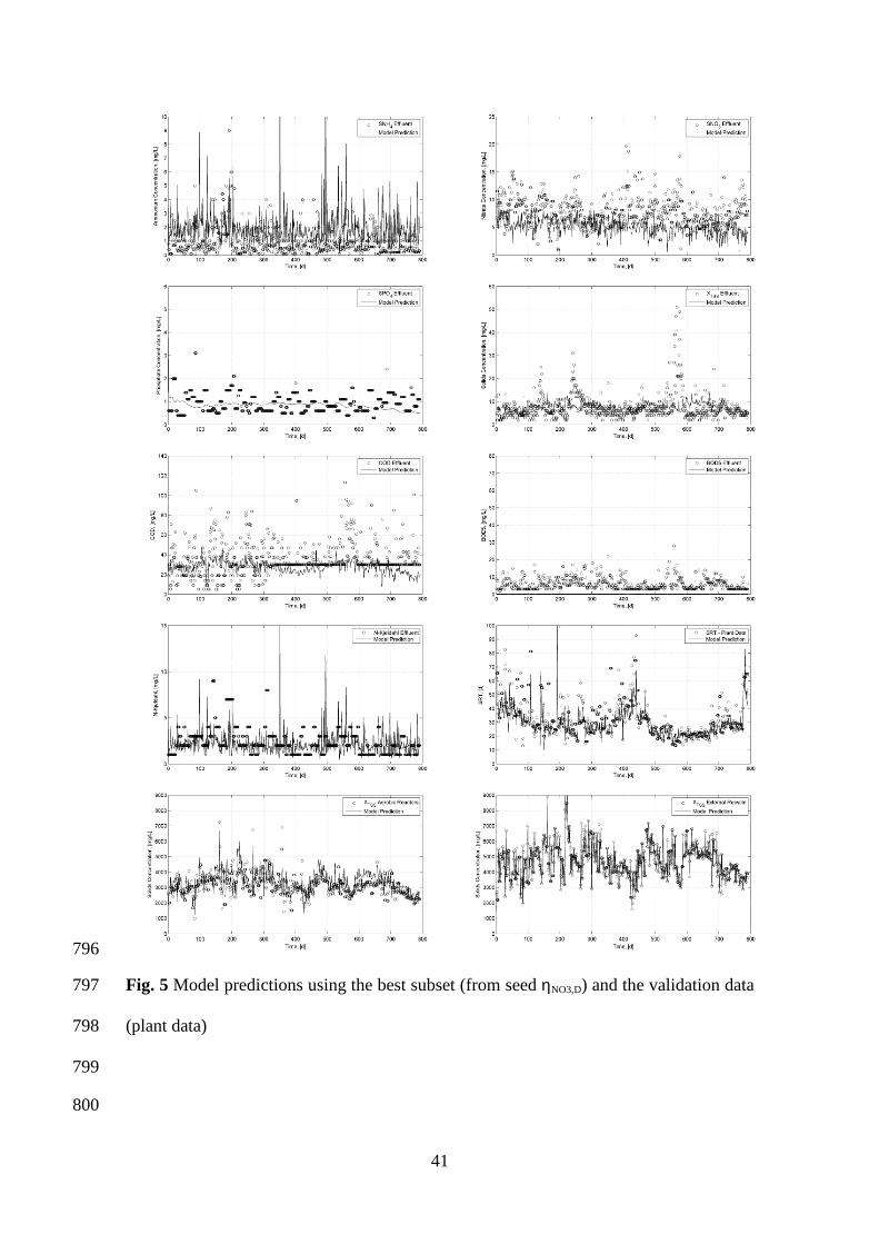
796
Fig. 5 Model predictions using the best subset (from seed ηNO3,D) and the validation data 797
(plant data) 798
799
800
42
Supplementary information 801
802
Activated Sludge Model 2d calibration with full-scale WWTP data: comparing 803
model parameter identifiability with influent and operational uncertainty. 804
805
Vinicius Cunha Machado, Javier Lafuente, Juan Antonio Baeza* 806
807
Department of Chemical Engineering, Universitat Autònoma de Barcelona, ETSE, 808
08193 Bellaterra (Barcelona), Spain. Phone: +34935811587. FAX: +34935812013. 809
E-mails: [email protected], [email protected], 810
*Corresponding Author 812
813

43
S1. Influent Characterization Procedure 814
Orhon et al. [1] developed a method to determine the values of SI, XI, XS and SF 815
(ASM2d states) in the effluent, using the well-know measurement of the COD. X 816
variables are the particulate variables while S variables indicate soluble variables. Such 817
method allows making an interface between the COD and ASM2d state variables. 818
The experimental determination of SI and XI is performed in two parallel CSTR reactors, 819
one of them fed with raw WWTP influent and the other one fed with filtered WWTP 820
influent. Both reactors operate as long as all the biological reactions have been ceased 821
and daily analysis of total COD and the soluble COD are performed. At a sufficient 822
time, both values of COD of the two systems will be approximately constant. At the end 823
of the experiment, the relationship between the initial and final values of total COD and 824
soluble COD of both systems will help to estimate SI and XI. 825
XS is present at the beginning of the experiment for reactor 1 (with raw influent, without 826
filtering) and it is not for reactor 2 (with filtered WW). At the end of the experiment, in 827
both systems XS and SF no longer exist, differently of SP and XP that are produced by the 828
microorganisms along the experiment time. SP and XP are, respectively, soluble and 829
particulate residual biodegradable matter, product of microorganism activity. XI is 830
present at the end of the experiment only in reactor 1 (no filtered WW). With these 831
observations, it is possible to write a system of equations as follows: 832
833
44
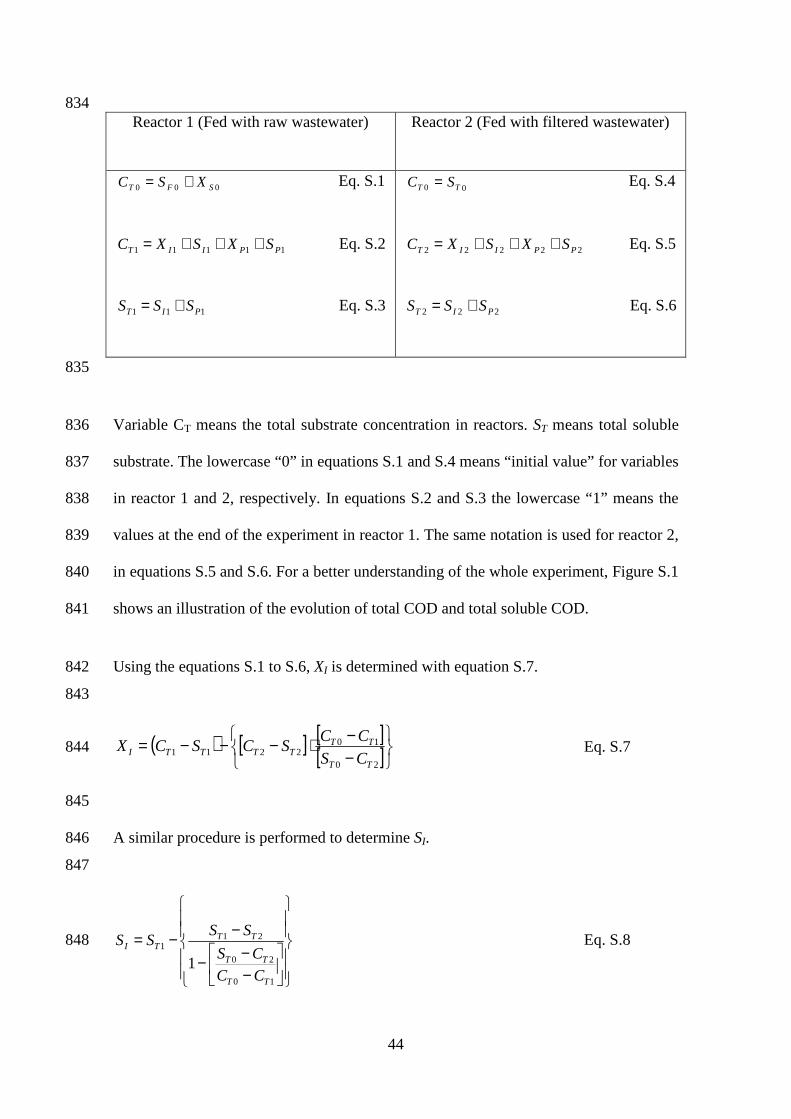
834 Reactor 1 (Fed with raw wastewater) Reactor 2 (Fed with filtered wastewater)
000 SFT XSC += Eq. S.1
11111 PPIIT SXSXC +++= Eq. S.2
111 PIT SSS += Eq. S.3
00 TT SC = Eq. S.4
22222 PPIIT SXSXC +++= Eq. S.5
222 PIT SSS += Eq. S.6
835
Variable CT means the total substrate concentration in reactors. ST means total soluble 836
substrate. The lowercase “0” in equations S.1 and S.4 means “initial value” for variables 837
in reactor 1 and 2, respectively. In equations S.2 and S.3 the lowercase “1” means the 838
values at the end of the experiment in reactor 1. The same notation is used for reactor 2, 839
in equations S.5 and S.6. For a better understanding of the whole experiment, Figure S.1 840
shows an illustration of the evolution of total COD and total soluble COD. 841
Using the equations S.1 to S.6, XI is determined with equation S.7. 842
843
( ) [ ] [ ][ ]
−−⋅−−−=
20
102211
TT
TTTTTTI CS
CCSCSCX Eq. S.7 844
845
A similar procedure is performed to determine SI. 846
847
−−−
−−=
10
20
211
1TT
TT
TTTI
CC
CS
SSSS Eq. S.8 848

45
SF value can be obtained by taking the value of total soluble COD of reactor 2 at the 849
beginning of the experiment for determining XI and SI and subtracting the value of SI 850
(obtained by Eq. S.8). 851
852
IF SCODS −= WW)(filteredSoluble Eq. S.9 853
Finally, XS is determined by using measures of total COD in reactor 1. 854
( )IIFAtotalS XSSS-DQOX +++= Eq. S.10 855
In Eq. S.10, SA should be considered null (no conditions of fermenting XS to produce SA 856
in the urban sewage system) and the rest of variables were already determined. 857
858
Aigua residual filtrada
Reactor No: 2
Aigua residual
Reactor No: 1
Aigua residual filtrada
Reactor No: 2
Aigua residual filtrada
Reactor No: 2
Aigua residual filtrada
Reactor No: 2
Aigua residual
Reactor No: 1
Aigua residual
Reactor No: 1
Aigua residual
Reactor No: 1
Aigua residual
Reactor No: 1
DQ
O (
mg
L-1)
0
200
400
600
800
1000
Col 2 vs Col 3 Col 2 vs Col 4
Temps (dies)
0 10 20 30 40 50 600
100
200
300
400
500Reactor Nº 2
Reactor Nº 1
∆CT2=ST0-CT2=SF0-SP2-XP2
CT2=SP2+SI+XP2
CT2-ST2=XP2
ST2=SP2+SI
∆CT1=CT0-CT1=CS0-SP1-XP1
CT1=SP1+SI+XP1+XI
CT1-ST1=XP1+XI
ST1=SP1+SI
DQ
O (
mg
L-1)
0
200
400
600
800
1000
Col 2 vs Col 3 Col 2 vs Col 4
Temps (dies)
0 10 20 30 40 50 600
100
200
300
400
500Reactor Nº 2
Reactor Nº 1
∆CT2=ST0-CT2=SF0-SP2-XP2
CT2=SP2+SI+XP2
CT2-ST2=XP2
ST2=SP2+SI
∆CT1=CT0-CT1=CS0-SP1-XP1
CT1=SP1+SI+XP1+XI
CT1-ST1=XP1+XI
ST1=SP1+SI
∆CT1=CT0-CT1=CS0-SP1-XP1
CT1=SP1+SI+XP1+XI
CT1-ST1=XP1+XI
ST1=SP1+SI
Figure S.1: Illustration of the lab scale reactors, total COD and total soluble COD data 859
for determining SI and XI fractions in the secondary stage influent in a WWTP 860
( • Total COD, ○ Total soluble COD). 861
862

46
S.2. Sensitivity Analysis 863
Sensitivity analysis allows making a ranking of the most important parameters that 864
affect the outputs. Relative sensitivity of an output i (yi) respect a parameter j (θj) is 865
defined as [2], 866
j
i
i
j
ji d
dy
yS
θθ
= Eq. S.11 867
Norton [3] proposed the utilization of algebraic sensitivity analysis because the 868
numerical value of sensitivity applies only for a specific change from a specific value of 869
θj, while the former provides algebraic relations. Numerical values of sensitivity are 870
generally much less informative than an algebraic relation, but algebraic sensitivity 871
analysis is not feasible if the equations of the model are complicated as in ASM2d. 872
Therefore, the derivatives of equation S.11 were determined numerically by the finite 873
differences method. The central difference approach with 10-4 (0.01%) as perturbation 874
factor was used for the sensitivity calculations of each tested parameter around the 875
default ASM2d value. This perturbation factor was selected because it produced equal 876
derivative values with forward and backward finite differences [4]. 877
The overall sensitivity of a parameter was calculated by adding absolute values of 878
individual sensitivities. In our case, 5 output variables were declared (phosphate, 879
ammonium, nitrate, TSS and TKN concentrations at the effluent). Hence, the overall 880
sensitivity value of a parameter j (OSj) was calculated with equation S.12. 881
TKNjXTSSjNOjNHjPOjj SSSSSOS ,,,,, 344++++=
Eq. S.12 882
883
884
885

47
S.3. The Fisher Information Matrix and Parameter Confidence Interval 886
The FIM summarizes the importance of each model parameter over the outputs, since it 887
measures the variation of output variables caused by a variation of model parameters [5, 888
6]. Algebraically, the FIM is represented by equation S.13. 889
)k(YQ)k(YFIM Tk
N
kθθ ⋅⋅= −
=∑ 1
1 Eq. S.13 890
For a FIM calculated for r output variables and p parameters, it is a p x p matrix, where 891
k represents each sampling data point, QK is the r x r covariance matrix of the 892
measurement noise, θ is the vector of p parameters, N is the total number of samples 893
and Yθ is the p x r output sensitivity function matrix, expressed by equation S.14. 894
0
),()( 0
θθ θ
θ
∂∂
=T
T tytY
Eq. S.14 895
where θ0 is the complete model parameter vector used for calculating the derivatives 896
and θT is the transposed parameter vector, which its elements are being studied. In the 897
present study, the derivative shown in equation S.14 was numerically obtained by finite 898
differences using a perturbation factor of 10-4 as in the sensitivity calculations. 899
Mathematically was proved that the FIM provides a lower bound of the parameter error 900
covariance matrix [7] as shown by equation S.15. 901
( ) 10cov −≥ FIMθ Eq. S.15 902
This FIM property was used for calculating the confidence interval ∆θj with equation 903
S.16 for a given parameter θj [8]. 904
)cov(, jpNj t θθ α −=∆ Eq. S.16 905
48
where t is the statistical t-student with α = 95% of confidence and N-p degrees of 906
freedom (number of experimental data points minus p parameters), and cov(θj) was 907
assumed as FIM-1jj. 908
As can be observed, the calculation of the parameter error covariance matrix using the 909
FIM involves its inversion. To be invertible, the FIM should have a determinant 910
different from zero and should not be ill-conditioned. To match these requirements any 911
pair of matrix columns should not be very similar. As each column of the matrix 912
represents a parameter, the determinant and the condition number of the FIM provides a 913
reasonable measurement of the correlation of a set of parameters. Hence, parameters 914
less correlated will easily provide a diagonal-dominant matrix. The FIM determinant (D 915
criterion) and the ratio between the highest and the lowest FIM eigenvalue (modE 916
criterion) can be used as criteria for parameter subset selection. A modE criterion value 917
close to the unity indicates that all the involved parameters independently affect the 918
outputs while the shape of the confidence region is similar to a circle (2 parameters) or a 919
sphere (3 parameters) and not ellipses and ellipsoids as occur with correlated 920
parameters. A high D criterion value means lower values of the diagonal elements of the 921
covariance matrix, and as a consequence, lower confidence intervals of the parameters. 922
As the D criterion is dependent on the magnitude of the involved parameters, this 923
criterion was normalized (normD) according to Equation S.17. 924
2
PθDnormD ⋅= Eq. S.17 925
where ||θP|| is the Euclidean norm of the parameter vector. Such normalization works as 926
a scaling factor and allows comparisons among subsets with the same size but with 927
different parameters. 928
From the system engineering point of view, it is important to include in the parameter 929
subset those parameters that maximize the D criterion and minimize the modE criterion. 930

49
Hence, the ratio between the normD and the modE criteria (RDE criterion) was 931
proposed [9] as an interesting index to define subsets of parameters for calibration. The 932
RDE criterion (Equation S.18) establishes the capacity of a parameter subset to explain 933
experimental data coupled to low uncertainty in the estimated parameters. 934
modE
normDRDE =
Eq. S.18 935
936
S.4. References 937
1. Orhon D, Artan N, Ates E (1994) A description of three methods for the 938 determination of the initial inert particulate chemical oxigen demand of 939 wastewater. J Chem Technol Biot 61:73–80 940
2. Reichert P, Vanrolleghem PA (2001) Identifiability and uncertainty analysis of 941 the river water quality model no. 1 (RWQM1). Water Sci Technol 43:329–338 942
3. Norton JP (2008) Algebraic sensitivity analysis of environmental models. 943 Environ Model Softw 23:963–972 944
4. De Pauw DJW (2005) Optimal Experimental Design for Calibration of 945 Bioprocess Models: A Validated Software Toolbox. PhD thesis in Applied 946 Biological Sciences. Available from: 947 http://biomath.ugent.be/publications/download/. University of Gent, Belgium 948
5. Dochain D, Vanrolleghem PA (2001) Dynamical modelling and estimation in 949 wastewater treatment processes. IWA Publishing, London 950
6. Guisasola A, Baeza JA, Carrera J, Sin G, Vanrolleghem PA, Lafuente J (2006) 951 The influence of experimental data quality and quantity on parameter estimation 952 accuracy. Education for Chemical Engineers 1:139–145 953
7. Söderström T, Stoica P (1989) System identification. Prentice-Hall, Englewood 954 Cliffs, New Jersey 955
8. Seber GAF, Wild CJ (1989) Nonlinear regression. Wiley, New York 956
9. Machado VC, Tapia G, Gabriel D, Lafuente J, Baeza JA (2009) Systematic 957 identifiability study based on the Fisher Information Matrix for reducing the 958 number of parameters calibration of an activated sludge model. Environ Model 959 Softw 24:1274–1284 960
961


![6. Activated Sludge Process : Introductionwemt.snu.ac.kr/lecture 2012-2/ENV/Ch 6/nCh 6 [호환 모드].pdf · 6. Activated Sludge Process : Introduction • The Activated sludge Process:](https://img.dokumen.tips/doc/110x75/5cc4ba0288c993ab2a8c5e09/6-activated-sludge-process-2012-2envch-6nch-6-pdf-6-activated.jpg)