Embed Size (px)
DESCRIPTION
09 - finite element method - density growth - implementation. 09 - finite element method. integration point based. loop over all time steps. global newton iteration. loop over all elements. loop over all quadrature points. local newton iteration to determine. - PowerPoint PPT Presentation
Citation preview
109 - finite element method
09 - finite element method -
density growth - implementation
2finite element method
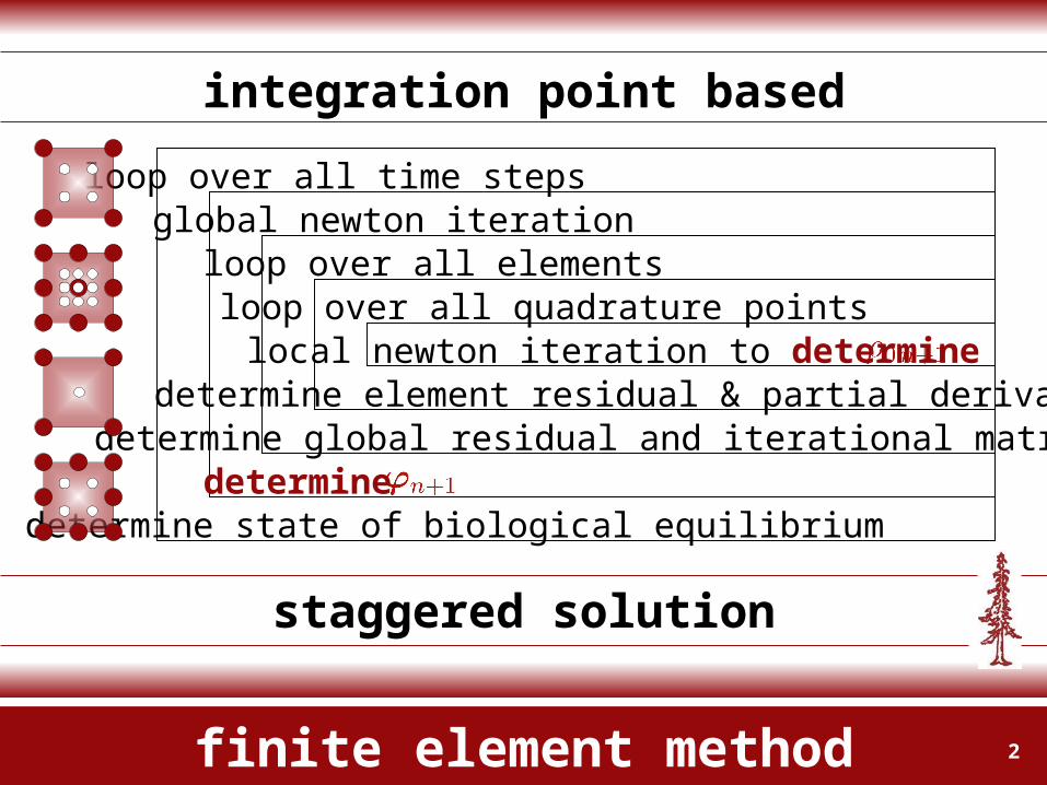
integration point based
staggered solution
loop over all time stepsglobal newton iteration
loop over all elementsloop over all quadrature pointslocal newton iteration to determine
determine element residual & partial derivativedetermine global residual and iterational matrixdetermine
determine state of biological equilibrium
3finite element method
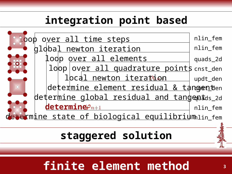
integration point based
staggered solution
loop over all time stepsglobal newton iteration
loop over all elementsloop over all quadrature points
local newton iterationdetermine element residual & tangent
determine global residual and tangentdetermine
determine state of biological equilibrium
nlin_fem
cnst_den
nlin_fem
quads_2d
updt_den
cnst_den
nlin_fem
nlin_fem
quads_2d
4finite element method
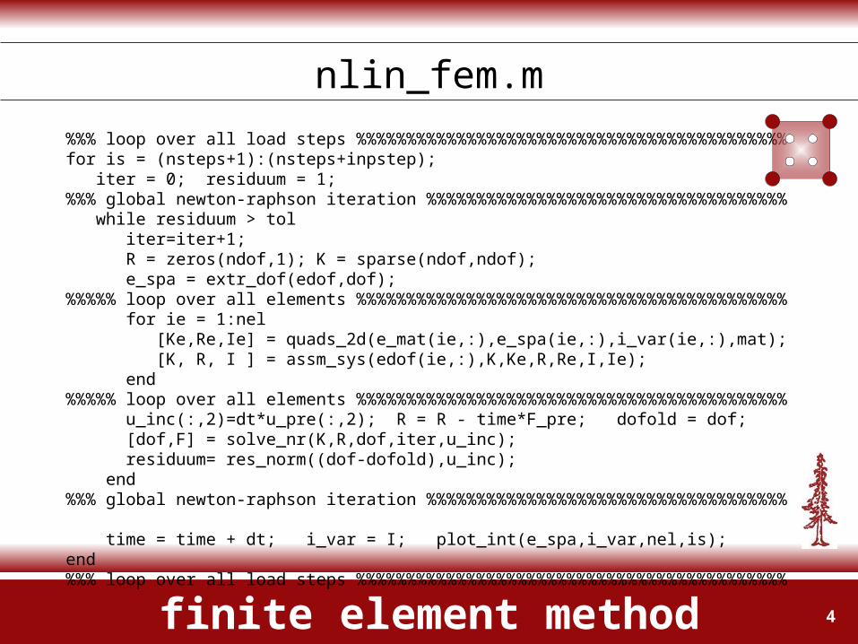
nlin_fem.m
%%% loop over all load steps %%%%%%%%%%%%%%%%%%%%%%%%%%%%%%%%%%%%%%%%%%%for is = (nsteps+1):(nsteps+inpstep); iter = 0; residuum = 1;%%% global newton-raphson iteration %%%%%%%%%%%%%%%%%%%%%%%%%%%%%%%%%%%% while residuum > tol iter=iter+1; R = zeros(ndof,1); K = sparse(ndof,ndof); e_spa = extr_dof(edof,dof); %%%%% loop over all elements %%%%%%%%%%%%%%%%%%%%%%%%%%%%%%%%%%%%%%%%%%% for ie = 1:nel [Ke,Re,Ie] = quads_2d(e_mat(ie,:),e_spa(ie,:),i_var(ie,:),mat); [K, R, I ] = assm_sys(edof(ie,:),K,Ke,R,Re,I,Ie); end%%%%% loop over all elements %%%%%%%%%%%%%%%%%%%%%%%%%%%%%%%%%%%%%%%%%%% u_inc(:,2)=dt*u_pre(:,2); R = R - time*F_pre; dofold = dof; [dof,F] = solve_nr(K,R,dof,iter,u_inc); residuum= res_norm((dof-dofold),u_inc); end%%% global newton-raphson iteration %%%%%%%%%%%%%%%%%%%%%%%%%%%%%%%%%%%% time = time + dt; i_var = I; plot_int(e_spa,i_var,nel,is);end %%% loop over all load steps %%%%%%%%%%%%%%%%%%%%%%%%%%%%%%%%%%%%%%%%%%%
5finite element method
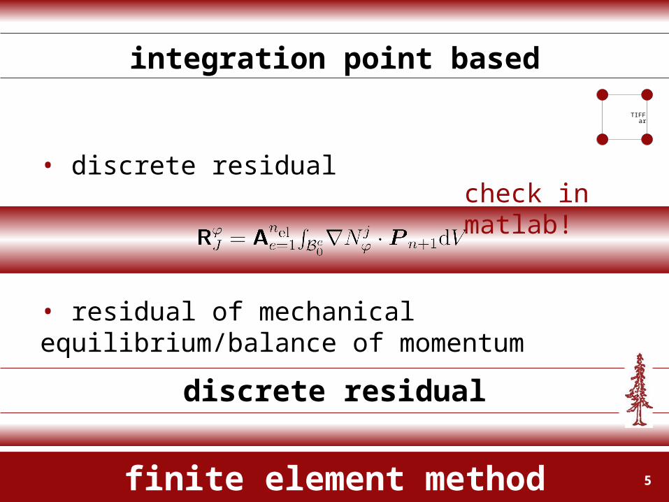
integration point based
discrete residual
• discrete residual
QuickTime™ and aTIFF (Uncompressed) decompressor
are needed to see this picture.
• residual of mechanical equilibrium/balance of momentum
check in matlab!
6finite element method
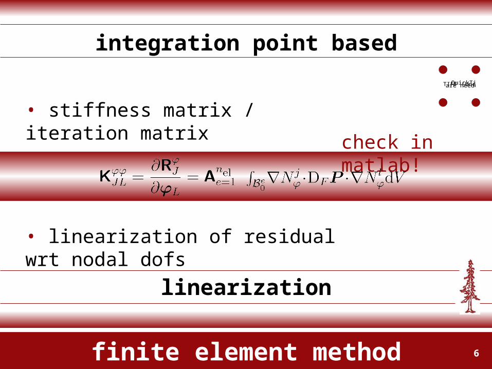
integration point based
linearization
• stiffness matrix / iteration matrix
QuickTime™ and aTIFF (Uncompressed) decompressorare needed to see this picture.
• linearization of residual wrt nodal dofs
check in matlab!
7finite element method
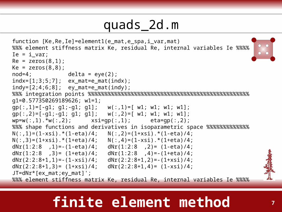
quads_2d.mfunction [Ke,Re,Ie]=element1(e_mat,e_spa,i_var,mat)%%% element stiffness matrix Ke, residual Re, internal variables Ie %%%% Ie = i_var;Re = zeros(8,1);Ke = zeros(8,8);nod=4; delta = eye(2);indx=[1;3;5;7]; ex_mat=e_mat(indx); indy=[2;4;6;8]; ey_mat=e_mat(indy); %%% integration points %%%%%%%%%%%%%%%%%%%%%%%%%%%%%%%%%%%%%%%%%%%%%%%%%g1=0.577350269189626; w1=1;gp(:,1)=[-g1; g1;-g1; g1]; w(:,1)=[ w1; w1; w1; w1]; gp(:,2)=[-g1;-g1; g1; g1]; w(:,2)=[ w1; w1; w1; w1];wp=w(:,1).*w(:,2); xsi=gp(:,1); eta=gp(:,2);%%% shape functions and derivatives in isoparametric space %%%%%%%%%%%%%N(:,1)=(1-xsi).*(1-eta)/4; N(:,2)=(1+xsi).*(1-eta)/4;N(:,3)=(1+xsi).*(1+eta)/4; N(:,4)=(1-xsi).*(1+eta)/4;dNr(1:2:8 ,1)=-(1-eta)/4; dNr(1:2:8 ,2)= (1-eta)/4;dNr(1:2:8 ,3)= (1+eta)/4; dNr(1:2:8 ,4)=-(1+eta)/4;dNr(2:2:8+1,1)=-(1-xsi)/4; dNr(2:2:8+1,2)=-(1+xsi)/4;dNr(2:2:8+1,3)= (1+xsi)/4; dNr(2:2:8+1,4)= (1-xsi)/4;JT=dNr*[ex_mat;ey_mat]';%%% element stiffness matrix Ke, residual Re, internal variables Ie %%%%
8finite element method
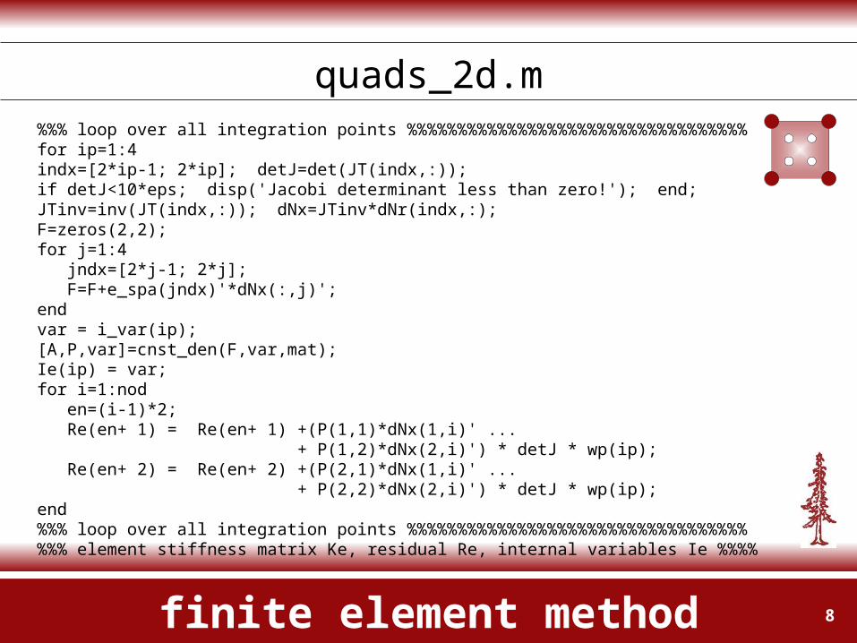
quads_2d.m%%% loop over all integration points %%%%%%%%%%%%%%%%%%%%%%%%%%%%%%%%%%for ip=1:4 indx=[2*ip-1; 2*ip]; detJ=det(JT(indx,:)); if detJ<10*eps; disp('Jacobi determinant less than zero!'); end; JTinv=inv(JT(indx,:)); dNx=JTinv*dNr(indx,:); F=zeros(2,2); for j=1:4 jndx=[2*j-1; 2*j]; F=F+e_spa(jndx)'*dNx(:,j)'; end var = i_var(ip); [A,P,var]=cnst_den(F,var,mat); Ie(ip) = var; for i=1:nod en=(i-1)*2; Re(en+ 1) = Re(en+ 1) +(P(1,1)*dNx(1,i)' ... + P(1,2)*dNx(2,i)') * detJ * wp(ip); Re(en+ 2) = Re(en+ 2) +(P(2,1)*dNx(1,i)' ... + P(2,2)*dNx(2,i)') * detJ * wp(ip); end %%% loop over all integration points %%%%%%%%%%%%%%%%%%%%%%%%%%%%%%%%%%%%% element stiffness matrix Ke, residual Re, internal variables Ie %%%%
9finite element method
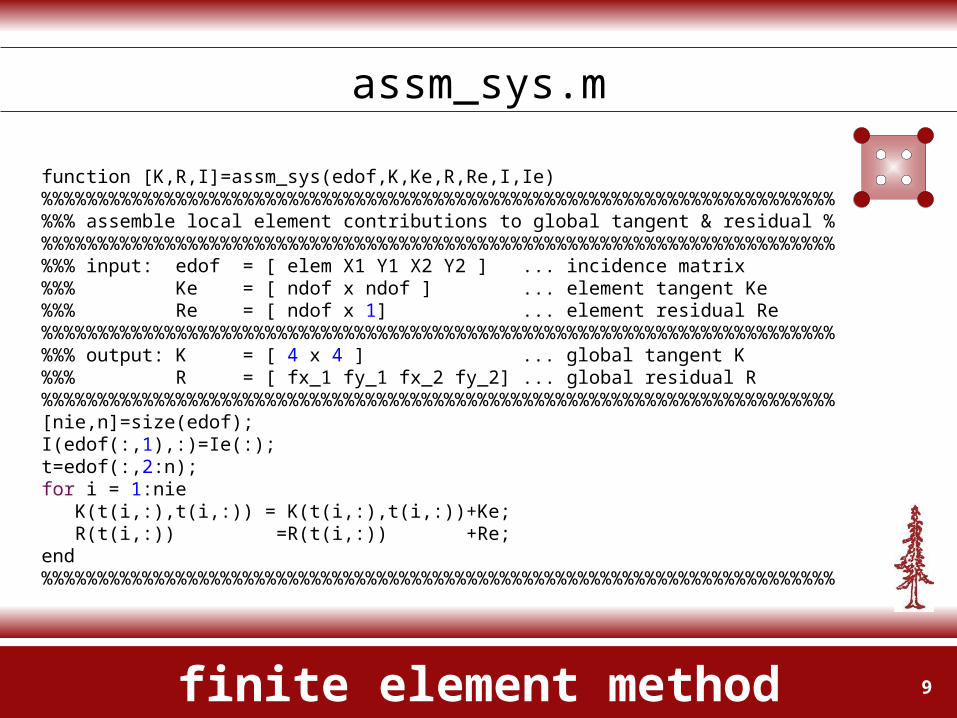
assm_sys.m
function [K,R,I]=assm_sys(edof,K,Ke,R,Re,I,Ie)%%%%%%%%%%%%%%%%%%%%%%%%%%%%%%%%%%%%%%%%%%%%%%%%%%%%%%%%%%%%%%%%%%%%%%%%%% assemble local element contributions to global tangent & residual %%%%%%%%%%%%%%%%%%%%%%%%%%%%%%%%%%%%%%%%%%%%%%%%%%%%%%%%%%%%%%%%%%%%%%%%%%% input: edof = [ elem X1 Y1 X2 Y2 ] ... incidence matrix%%% Ke = [ ndof x ndof ] ... element tangent Ke%%% Re = [ ndof x 1] ... element residual Re%%%%%%%%%%%%%%%%%%%%%%%%%%%%%%%%%%%%%%%%%%%%%%%%%%%%%%%%%%%%%%%%%%%%%%%%%% output: K = [ 4 x 4 ] ... global tangent K%%% R = [ fx_1 fy_1 fx_2 fy_2] ... global residual R%%%%%%%%%%%%%%%%%%%%%%%%%%%%%%%%%%%%%%%%%%%%%%%%%%%%%%%%%%%%%%%%%%%%%%%[nie,n]=size(edof);I(edof(:,1),:)=Ie(:);t=edof(:,2:n);for i = 1:nie K(t(i,:),t(i,:)) = K(t(i,:),t(i,:))+Ke; R(t(i,:)) =R(t(i,:)) +Re;end%%%%%%%%%%%%%%%%%%%%%%%%%%%%%%%%%%%%%%%%%%%%%%%%%%%%%%%%%%%%%%%%%%%%%%%
10finite element method
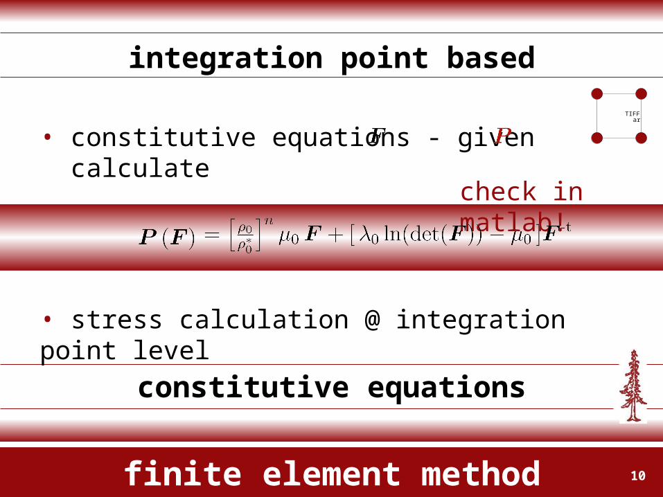
integration point based
constitutive equations
• stress calculation @ integration point level
QuickTime™ and aTIFF (Uncompressed) decompressor
are needed to see this picture.
• constitutive equations - given calculate
check in matlab!
11finite element method
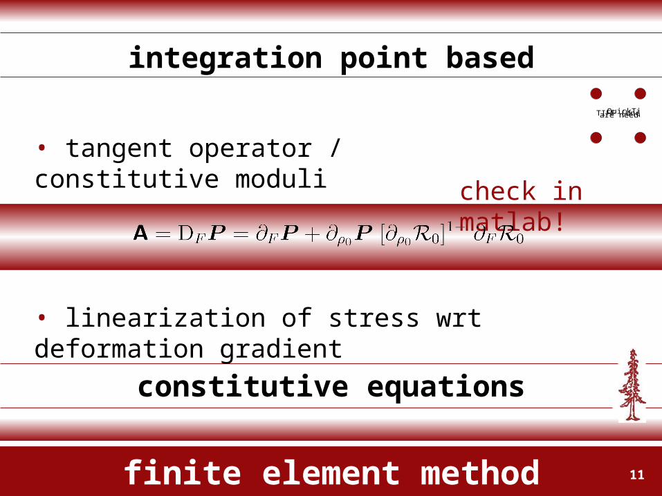
integration point based
constitutive equations
• tangent operator / constitutive moduli
QuickTime™ and aTIFF (Uncompressed) decompressorare needed to see this picture.
• linearization of stress wrt deformation gradient
check in matlab!
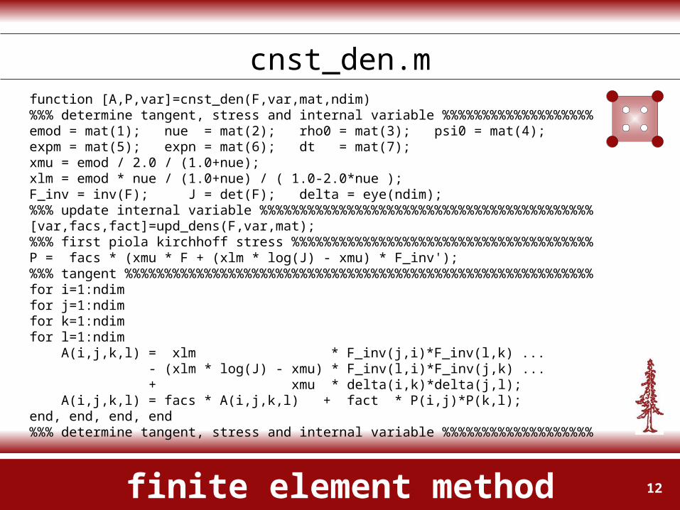
12finite element method
cnst_den.mfunction [A,P,var]=cnst_den(F,var,mat,ndim)%%% determine tangent, stress and internal variable %%%%%%%%%%%%%%%%%%%emod = mat(1); nue = mat(2); rho0 = mat(3); psi0 = mat(4); expm = mat(5); expn = mat(6); dt = mat(7);xmu = emod / 2.0 / (1.0+nue);xlm = emod * nue / (1.0+nue) / ( 1.0-2.0*nue ); F_inv = inv(F); J = det(F); delta = eye(ndim);%%% update internal variable %%%%%%%%%%%%%%%%%%%%%%%%%%%%%%%%%%%%%%%%%%[var,facs,fact]=upd_dens(F,var,mat); %%% first piola kirchhoff stress %%%%%%%%%%%%%%%%%%%%%%%%%%%%%%%%%%%%%%P = facs * (xmu * F + (xlm * log(J) - xmu) * F_inv'); %%% tangent %%%%%%%%%%%%%%%%%%%%%%%%%%%%%%%%%%%%%%%%%%%%%%%%%%%%%%%%%%%for i=1:ndimfor j=1:ndimfor k=1:ndimfor l=1:ndim A(i,j,k,l) = xlm * F_inv(j,i)*F_inv(l,k) ... - (xlm * log(J) - xmu) * F_inv(l,i)*F_inv(j,k) ... + xmu * delta(i,k)*delta(j,l); A(i,j,k,l) = facs * A(i,j,k,l) + fact * P(i,j)*P(k,l); end, end, end, end%%% determine tangent, stress and internal variable %%%%%%%%%%%%%%%%%%%

13finite element method
integration point based
constitutive equations
QuickTime™ and aTIFF (Uncompressed) decompressor
are needed to see this picture.
check in matlab!
• residual of biological equilibrium / balance of mass
• discrete density update
14finite element method
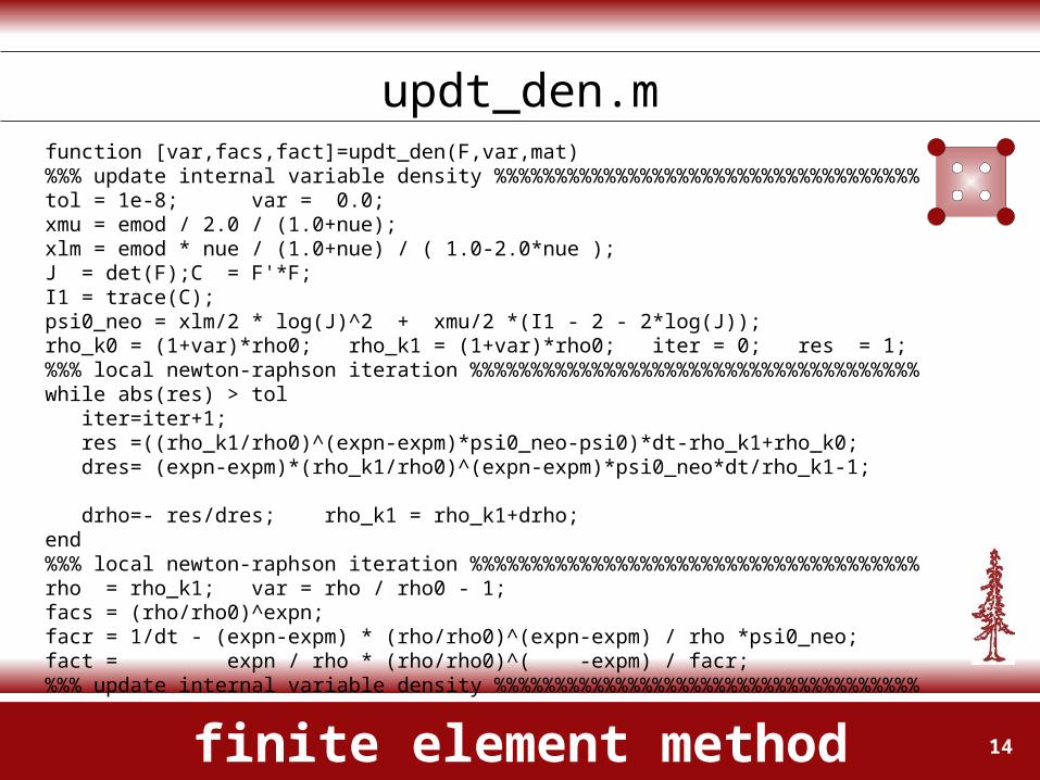
updt_den.mfunction [var,facs,fact]=updt_den(F,var,mat)%%% update internal variable density %%%%%%%%%%%%%%%%%%%%%%%%%%%%%%%%%%%tol = 1e-8; var = 0.0;xmu = emod / 2.0 / (1.0+nue);xlm = emod * nue / (1.0+nue) / ( 1.0-2.0*nue ); J = det(F);C = F'*F;I1 = trace(C);psi0_neo = xlm/2 * log(J)^2 + xmu/2 *(I1 - 2 - 2*log(J)); rho_k0 = (1+var)*rho0; rho_k1 = (1+var)*rho0; iter = 0; res = 1;%%% local newton-raphson iteration %%%%%%%%%%%%%%%%%%%%%%%%%%%%%%%%%%%%% while abs(res) > tol iter=iter+1; res =((rho_k1/rho0)^(expn-expm)*psi0_neo-psi0)*dt-rho_k1+rho_k0; dres= (expn-expm)*(rho_k1/rho0)^(expn-expm)*psi0_neo*dt/rho_k1-1; drho=- res/dres; rho_k1 = rho_k1+drho; end%%% local newton-raphson iteration %%%%%%%%%%%%%%%%%%%%%%%%%%%%%%%%%%%%% rho = rho_k1; var = rho / rho0 - 1;facs = (rho/rho0)^expn;facr = 1/dt - (expn-expm) * (rho/rho0)^(expn-expm) / rho *psi0_neo;fact = expn / rho * (rho/rho0)^( -expm) / facr;%%% update internal variable density %%%%%%%%%%%%%%%%%%%%%%%%%%%%%%%%%%%
15finite element method
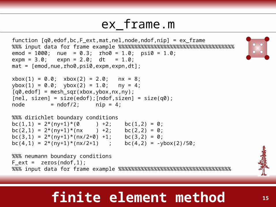
ex_frame.mfunction [q0,edof,bc,F_ext,mat,nel,node,ndof,nip] = ex_frame%%% input data for frame example %%%%%%%%%%%%%%%%%%%%%%%%%%%%%%%%%%%%emod = 1000; nue = 0.3; rho0 = 1.0; psi0 = 1.0;expm = 3.0; expn = 2.0; dt = 1.0;mat = [emod,nue,rho0,psi0,expm,expn,dt];
xbox(1) = 0.0; xbox(2) = 2.0; nx = 8; ybox(1) = 0.0; ybox(2) = 1.0; ny = 4;[q0,edof] = mesh_sqr(xbox,ybox,nx,ny); [nel, sizen] = size(edof);[ndof,sizen] = size(q0); node = ndof/2; nip = 4;
%%% dirichlet boundary conditionsbc(1,1) = 2*(ny+1)*(0 ) +2; bc(1,2) = 0;bc(2,1) = 2*(ny+1)*(nx ) +2; bc(2,2) = 0; bc(3,1) = 2*(ny+1)*(nx/2+0) +1; bc(3,2) = 0; bc(4,1) = 2*(ny+1)*(nx/2+1) ; bc(4,2) = -ybox(2)/50;
%%% neumann boundary conditionsF_ext = zeros(ndof,1);%%% input data for frame example %%%%%%%%%%%%%%%%%%%%%%%%%%%%%%%%%%%
16finite element method
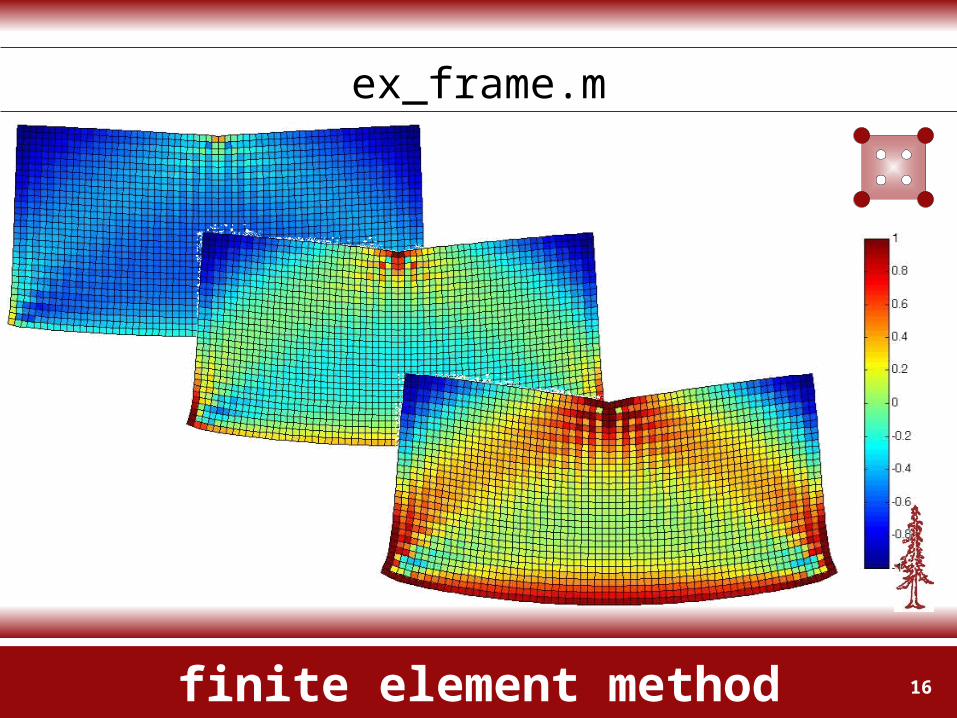
ex_frame.m

17finite element method
ex_femur.mfunction [q0,edof,emat,bc,F_ext,mat,ndim,nel,node,ndof,nip,nlod] = ex_frame%%% input data for femur example %%%%%%%%%%%%%%%%%%%%%%%%%%%%%%%%%%%%%%%%%%%emod = 500; nue = 0.2; rho0 = 1.0; psi0 = 0.01;expm = 3.0; expn = 2.0; dt = 5.0;mat = [emod,nue,rho0,psi0,expm,expn,dt];
[q0,edof]=in_femur;[nel,sizen] = size(edof); [ndof,sizen] = size(q0); for ie=1:nel emat(ie) = 1; end; node = ndof/2; nip = 4; ndim = 2;%%%%%%%%%%%%%%%%%%%%%%%%%%%%%%%%%%%%%%%%%%%%%%%%%%%%%%%%%%%%%%%%%%%%%%%%%%%% dirichlet boundary conditionsbc(1,1) = 1; bc(1,2) = 0; bc(2,1) = 2; bc(2,2) = 0; for i=2:15 bc(i+1,1) = 2*i; bc(i+1,2) = 0; end;%%%%%%%%%%%%%%%%%%%%%%%%%%%%%%%%%%%%%%%%%%%%%%%%%%%%%%%%%%%%%%%%%%%%%%%%%%%% neumann boundary conditionsF_ext = zeros(ndof,1); F_ext(372*2-1)= 0.5496; F_ext(372*2)= 1.3517; % load case 1,2,3F_ext(692*2-1)= 0.2997; F_ext(692*2)=-1.1185; % load case 2F_ext(720*2-1)=-1.2792; F_ext(720*2)=-0.8628; % load case 3F_ext(723*2-1)=-0.9424; F_ext(723*2)=-2.1167; % load case 1%%% input data for frame example %%%%%%%%%%%%%%%%%%%%%%%%%%%%%%%%%%%%%%%%%%
18finite element method
ex_femur.m
QuickTime™ and aTIFF (Uncompressed) decompressor
are needed to see this picture.
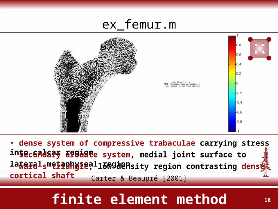
• dense system of compressive trabaculae carrying stress into calcar region• secondary arcuate system, medial joint surface to lateral metaphyseal region• ward‘s triangle, low density region contrasting dense cortical shaft Carter & Beaupré [2001]


