0124852 2005 postextual - DBD PUC RIO€¦ · 77 . scintillation for free-space laser communication at 785 nm and 1550 nm. Proc. Of SPIE Reprint, Vol 3850, 22 Sept 1999, Boston -

Bibliografia.

[1] IEC825; Safety of Laser Products. Equipment classification, requirements

and users guide . 1993.

[2] EARDLEY, P; WISELY, D; 1 Gb/s Optical Free Space Link Operating

over 40 m – System and Applications , IEE Proc. Optoelect., Special Issue

on Free Space Optical Communications, Dec. 1995.

[3] WISELY, D et al.; 4 km terrestrial line of sight optical free space link

operating at 155Mb/s; Proc. Free Space Laser Commun. Tech. VI, SPIE vol

2123, 1994.

[4] Canon U.S.A. ; Disponivel em

<http://www.usa.canon.com/html/industrial_canobeam/canobeam/index.html

>; acesso em: agosto 2004.

[5] Free Space Optics – Optical Wireless Laser Infrared Communication System

<http://www.cablefree.co.uk>; acesso em: setembro 2003.

[6] Lightpointe <http://www.lightpointe.com>; acesso em: agosto 2002.

[7] MOURA, L; ALHO Jr., M; RIBEIRO,R; Análise e Dimensionamento de

Sistemas Ópticos no Espaço Livre , Projeto Final, Dept. de Engenharia de

Telecomunicações, Niterói, Fevereiro 2003

[8] RICKLIN, Jennifer C.; Free-Space Laser Communication Using a Partially

Coherent Source Beam, Baltimore, Maryland, March 2002, Dissertation of

Doctor of Philosophy, Johns Hopkins University, p 3-5.

[9] ESA PORTAL; Press Releases, N° 69-2001: A world first : data

transmission between European satellites using laser light. Disponivel em

<http://www.esa.int/export/esaCP/Pr_69_2001_p_EN.html>; acesso em:

janeiro 2003.

[10] IRDA(Infrared Communication System Associate); Merit of Infrared

Communication Infrared Communication applied in such a place!

Disponivel em <http://www.icsa.gr.jp/english/e_article_007.htm>; acesso em:

janeiro 2003.

[11] KIM, Isaac I.; MITCHELL, Mary; KOREVAAR, Eric; Measurement of

DBD

PUC-Rio - Certificação Digital Nº 0124852/CA

77

scintillation for free-space laser communication at 785 nm and 1550 nm.

Proc. Of SPIE Reprint, Vol 3850, 22 Sept 1999, Boston - Massachusetts

[12] SZWEDA, Roy (Associate Editor); “Laser for free-space optical

communications”, III-Vs Review, The Advanced Semiconductor Magazine,

Vol 14 – N° 8, pp. 46-49, October 2001.

[13] CARLSON, Robert T.; Reliability and availability in free-space optical

systems, Optics in Information Systems – Optical Wireless Communications

Edited by Nabeel Riza, October 2001, vol 12 No 2 page 5.

[14] LIU, M., HILL, S.L.; Free Space Point to Point Laser and Optical

Communications. Disponivel em

<http://www.cms.livjm.ac.uk/pgnet2001/papers/mliu.doc>; acesso em janeiro 2003

[15] BERTOLOTTI, M.; Effects of Atmosphere on the Propagation of Laser

Beams, Laser And Their Applications, Editor A. Sona, Gordon & Breach,

New York, 1976, page 349 - 413.

[16] KIM, Isaac I. et al; Wireless optical transmission of fast ethernet, FDDI,

ATM, and ESCON protocol data using the TerraLink laser communication

system, Opt. Eng. 37(12) 3143-3155 (December 1998)

[17] KIM, Isaac I.; KOREVAAR, Eric; Availability of Free Space Optics (FSO) and

hybrid FSO/RF systems . Disponivel em

<http://www.freespaceoptic.com/WhitePapers/SPIE2001b.pdf>; acesso em: abril

2003.

[18] PIERCE, R.M; RAMAPRASAD, Jaya; EISENBERG, Eric; Optical

attenuation in fog and clouds, Optical Wireless Communication IV, Eric J.

Korevaar Editor, Proceeding of SPIE Vol 4530 68 (2001)

[19] CLARK, Gerlad; WILLEBRAND, Heinz; ACHOUR, Maha; Hybrid free

space optical/microwave communication networks: A unique solution for

ultra high-speed local loop connectivity. Disponivel em

<http://www.lightpointe.com/pdf/wp_hybrid_fso_microwave_comm_nets.pdf

>; acesso em: abril 2003.

[20] JETANATHAN, Muthu; IONOV, Pavel; Multi-Gigabits-per-second Optical

Wireless Communications . Diponivel em

http://freespaceoptic.com/WhitePapers/Jeganathan%20%20(Optical%20Crossing).

pdf; acesso em: agosto 2002.

DBD


78

[21] KIM, Isaac I.; McARTHUR, Bruce; KOREVAAR, Eric; Comparison of laser

beam propagation at 785 nm and 1550 nm in fog and haze for optical

wireless communications . Disponivel em

http://www.freespaceoptic.com/WhitePapers/Comparison_Of_Beam_in_Fog.pdf

; acesso em: agosto 2002;

[22] LAVEN, Philip; The Optics of the water drop The Mie and the Debye

series. Disponivel em < http://www.philiplaven.com/index1.html>; acesso

em: novembro 2003.

[23] WILLEBRAND, Heinz; GHUMAN, Baksheesh S.; Free-Space Optics:

Enabling Optical Connectivity in Today’s Networks, Sams Publishing,

Indianapolis, Indiana, Usa, 2002.

[24] CHU, T.S.; HOGG, D.C.; Effects of Precipitation on Propagation at 0.63, 3.5,

and 10.6 Microns, Bell System Technical Journal, May-June 1968, pp 723 –

759.

[25] SANCHEZ, L.J. et al.; Efficiency of off-axis astronomical adaptative systems:

comparison of experimental data for different astronomical sites, Adaptive

Optics System Technologies, SPIE Proc. 4007, Munich, Ed. P.L. Wizinowich,

pp. 749 – 755, 2000.

[26] CLIFFORD, S.F.; The Classical Theory of Wave Propagation in a Turbulent

Medium, Laser Beam Propagation in the Atmosphere, Topics in Applied

Physics, Vol. 25, pp. 9-43, Editor: J.W. Strohbehn, Springer-Verlag, Berlin-

Germany, 1978.

[27] FLACH, P.; Analysis of refraction influences in geodesy using image

processing and turbulence models. A dissertation submitted to the SWISS

FEDERAL INSTITUTE OF TECHNOLOGY ZURICH for the degree of

Doctor of Technical Sciences, Zurich, 2000, pp 83-84

[28] TATARSKI, Valerian Ilich; Wave propagation in a turbulent medium,

New York : Dover Publ., 1967. xiv,if.,285p.,7f. Dover books on physics and

mathematical physics Notas "Esta 1. ed. da Dover Publication é uma

reimpressão da tradução inglêsa publicada em 1961 pela McGraw-Hill Book

Company" (ver para este caso o capítulo 12).

[29] YURA, H.T.; McKINLEY, W.G.; Optical scintillation statistics for IR

ground-to-space laser communication systems, Applied Optics 22, 3353-3358

(1983).

DBD


79

[30] BELMONTE, A. et al.; Atmospheric-turbulence-induced power-fade statistics

for a multiaperture optical receiver , Applied Optics 36, 8632-8638 (1997).

[31] KOREVAAR, Eric et al.; Atmospheric Propagation Characteristics of

Highest Importance to Commercial Free Space Optics. Disponivel em

<http://www.mrv.com/library/library.php?ctl=MRV-WP-FSOAtmosProp.>;

acesso em: novembro 2003;

[32] HARBOE, P.B.; SOUZA, J.R.; Sistemas Ópticos no Espaço Livre: Estudo da

Viabilidade de Implementação em Cidade Brasileiras; XX Simpósio Brás. de

Telecomunicações – SBT´03, 05-08 Outubro 2003, Rio de Janeiro.

[33] KIM I.I. et al.; Measurement of scintillation and link margin for the

TerraLink laser communication system, Wireless Technologies and

System: Millimeter Wave and Optical, Proc. SPIE, Vol 3232, pp 100-118,

1997.

[34] PODCAMENI, A. <[email protected]> FSO Cetuc 20/05/2002.

22/maio/2002. Comunicação pessoal.

[35] BISWAS, A., LEE, S. Ground-to-ground optical communications

demonstrations , TMO Progress Report 42-141; May 15, 2000.

[36] PODCAMENI, A. <[email protected]> Registro de desempenho.

4/dezembro/2002. Comunicação pessoal.

[37] BLOOM, Scott et al.; Understanding the Performance of Free-Space Optics,

WCA Technical Symposium, San Jose, CA, January 14, 2003.

[38] ITU-T, G.826(02/99) Error performance parameters and objetives for

international, constant bit rate digital paths at or above the primary rate,

15th of February 1999.

[39] DERICKSON, Dennis; Fiber optic test and measurement, Cap 8, Upper

Saddle River, N. J., Prentice Hall,1998.

[40] ACTERNA; Recommendation G.826: Error Performance Parameters and

Objetives for International, Constant Bit Rate Digital Paths at or above the

Primary Rate.; ITU-T Recommendations and Practical Applicatins in

PDH/SDH Networks, Application Note 59, Wander & Goltermann

Communication Test Solution, Printed in Germany, page 12-13.

[41]TEKTRONIX; Synchronous Optical Network (SONET). Disponivel em

<http://www.iec.org/cgi-bin/acrobat.pl?filecode=131>; acesso em: dezembro

2002.

DBD


80

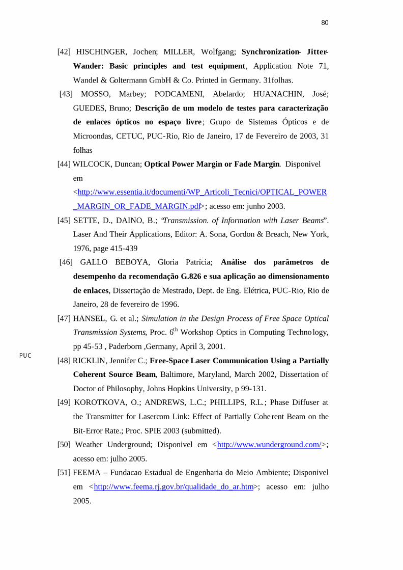
[42] HISCHINGER, Jochen; MILLER, Wolfgang; Synchronization- Jitter-

Wander: Basic principles and test equipment, Application Note 71,

Wandel & Goltermann GmbH & Co. Printed in Germany. 31folhas.

[43] MOSSO, Marbey; PODCAMENI, Abelardo; HUANACHIN, José;

GUEDES, Bruno; Descrição de um modelo de testes para caracterização

de enlaces ópticos no espaço livre ; Grupo de Sistemas Ópticos e de

Microondas, CETUC, PUC-Rio, Rio de Janeiro, 17 de Fevereiro de 2003, 31

folhas

[44] WILCOCK, Duncan; Optical Power Margin or Fade Margin. Disponivel

em

<http://www.essentia.it/documenti/WP_Articoli_Tecnici/OPTICAL_POWER

_MARGIN_OR_FADE_MARGIN.pdf>; acesso em: junho 2003.

[45] SETTE, D., DAINO, B.; “Transmission. of Information with Laser Beams”.

Laser And Their Applications, Editor: A. Sona, Gordon & Breach, New York,

1976, page 415-439

[46] GALLO BEBOYA, Gloria Patrícia; Análise dos parâmetros de

desempenho da recomendação G.826 e sua aplicação ao dimensionamento

de enlaces, Dissertação de Mestrado, Dept. de Eng. Elétrica, PUC-Rio, Rio de

Janeiro, 28 de fevereiro de 1996.

[47] HANSEL, G. et al.; Simulation in the Design Process of Free Space Optical

Transmission Systems, Proc. 6th Workshop Optics in Computing Techno logy,

pp 45-53 , Paderborn ,Germany, April 3, 2001.

[48] RICKLIN, Jennifer C.; Free-Space Laser Communication Using a Partially

Coherent Source Beam, Baltimore, Maryland, March 2002, Dissertation of

Doctor of Philosophy, Johns Hopkins University, p 99-131.

[49] KOROTKOVA, O.; ANDREWS, L.C.; PHILLIPS, R.L.; Phase Diffuser at

the Transmitter for Lasercom Link: Effect of Partially Coherent Beam on the

Bit-Error Rate.; Proc. SPIE 2003 (submitted).

[50] Weather Underground; Disponivel em <http://www.wunderground.com/>;

acesso em: julho 2005.

[51] FEEMA – Fundacao Estadual de Engenharia do Meio Ambiente; Disponivel

em <http://www.feema.rj.gov.br/qualidade_do_ar.htm>; acesso em: julho

2005.

DBD


81

Anexo A. Distribuição de Probabilidade LogNormal

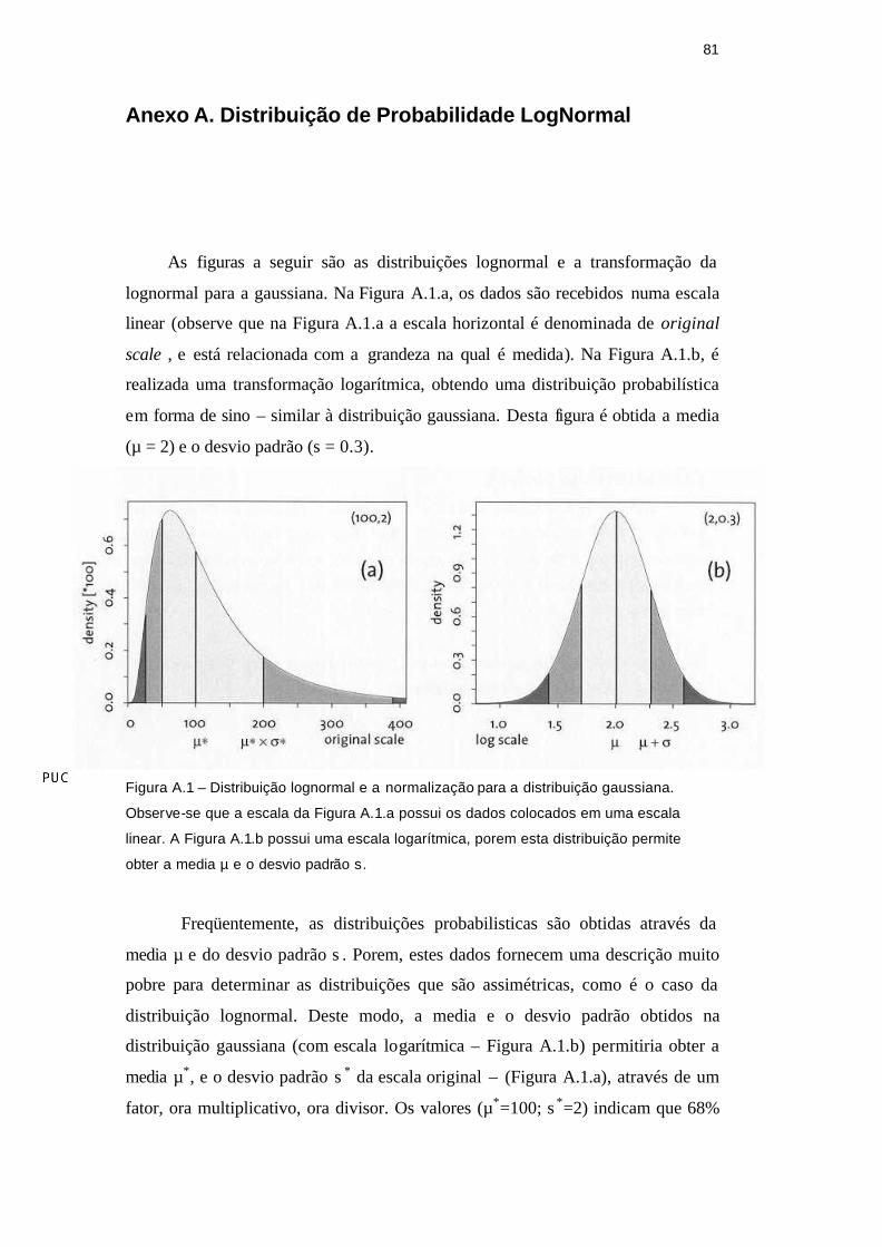
As figuras a seguir são as distribuições lognormal e a transformação da

lognormal para a gaussiana. Na Figura A.1.a, os dados são recebidos numa escala

linear (observe que na Figura A.1.a a escala horizontal é denominada de original

scale , e está relacionada com a grandeza na qual é medida). Na Figura A.1.b, é

realizada uma transformação logarítmica, obtendo uma distribuição probabilística

em forma de sino – similar à distribuição gaussiana. Desta figura é obtida a media

(µ = 2) e o desvio padrão (s = 0.3).

Figura A.1 – Distribuição lognormal e a normalização para a distribuição gaussiana.

Observe-se que a escala da Figura A.1.a possui os dados colocados em uma escala

linear. A Figura A.1.b possui uma escala logarítmica, porem esta distribuição permite

obter a media µ e o desvio padrão s.

Freqüentemente, as distribuições probabilisticas são obtidas através da

media µ e do desvio padrão s . Porem, estes dados fornecem uma descrição muito

pobre para determinar as distribuições que são assimétricas, como é o caso da

distribuição lognormal. Deste modo, a media e o desvio padrão obtidos na

distribuição gaussiana (com escala logarítmica – Figura A.1.b) permitiria obter a

media µ*, e o desvio padrão s * da escala original – (Figura A.1.a), através de um

fator, ora multiplicativo, ora divisor. Os valores (µ*=100; s *=2) indicam que 68%

DBD


82

da distribuição lognormal encontram-se entre os valores de [100 / 2 = 50 ; 100 x 2

= 200]. Os valores que compreendem o 95% da distribuição lognormal encontram-

se entre [ 100 / 22 = 25; 100 x 22 = 400].

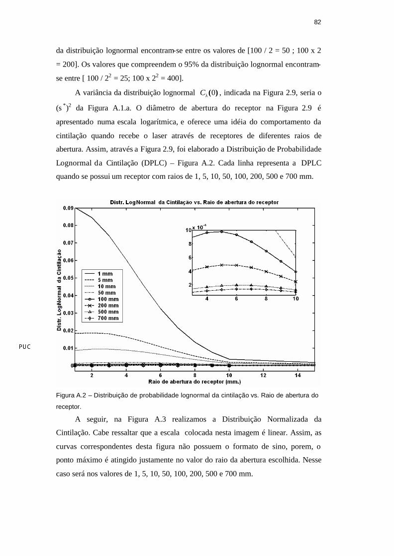
A variância da distribuição lognormal )(0λC , indicada na Figura 2.9, seria o

(s *)2 da Figura A.1.a. O diâmetro de abertura do receptor na Figura 2.9 é

apresentado numa escala logarítmica, e oferece uma idéia do comportamento da

cintilação quando recebe o laser através de receptores de diferentes raios de

abertura. Assim, através a Figura 2.9, foi elaborado a Distribuição de Probabilidade

Lognormal da Cintilação (DPLC) – Figura A.2. Cada linha representa a DPLC

quando se possui um receptor com raios de 1, 5, 10, 50, 100, 200, 500 e 700 mm.

Figura A.2 – Distribuição de probabilidade lognormal da cintilação vs. Raio de abertura do

receptor.

A seguir, na Figura A.3 realizamos a Distribuição Normalizada da

Cintilação. Cabe ressaltar que a escala colocada nesta imagem é linear. Assim, as

curvas correspondentes desta figura não possuem o formato de sino, porem, o

ponto máximo é atingido justamente no valor do raio da abertura escolhida. Nesse

caso será nos valores de 1, 5, 10, 50, 100, 200, 500 e 700 mm.

DBD


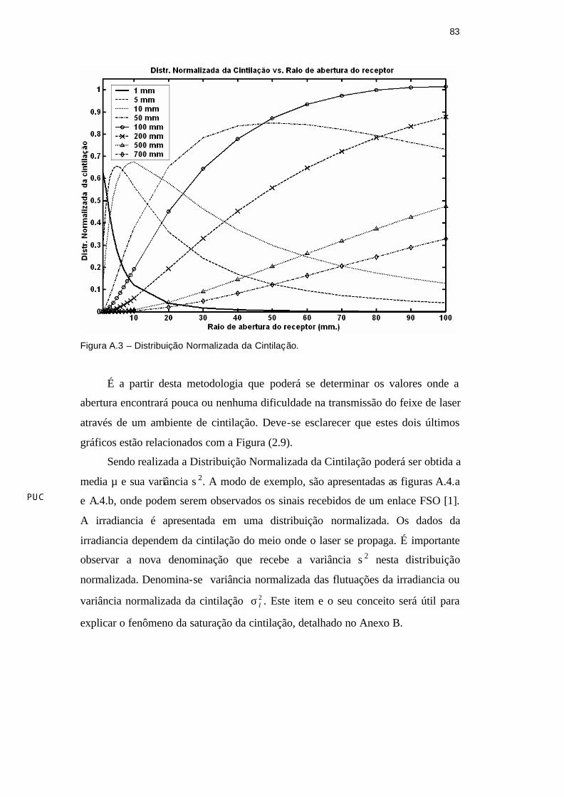
83

Figura A.3 – Distribuição Normalizada da Cintilação.

É a partir desta metodologia que poderá se determinar os valores onde a

abertura encontrará pouca ou nenhuma dificuldade na transmissão do feixe de laser

através de um ambiente de cintilação. Deve-se esclarecer que estes dois últimos

gráficos estão relacionados com a Figura (2.9).

Sendo realizada a Distribuição Normalizada da Cintilação poderá ser obtida a

media µ e sua variância s 2. A modo de exemplo, são apresentadas as figuras A.4.a

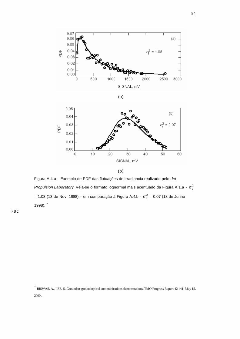
e A.4.b, onde podem serem observados os sinais recebidos de um enlace FSO [1].

A irradiancia é apresentada em uma distribuição normalizada. Os dados da

irradiancia dependem da cintilação do meio onde o laser se propaga. É importante

observar a nova denominação que recebe a variância s 2 nesta distribuição

normalizada. Denomina-se variância normalizada das flutuações da irradiancia ou

variância normalizada da cintilação 2Iσ . Este item e o seu conceito será útil para

explicar o fenômeno da saturação da cintilação, detalhado no Anexo B.

DBD


84

(a)

(b)

Figura A.4.a – Exemplo de PDF das flutuações de irradiancia realizado pelo Jet

Propulsion Laboratory. Veja-se o formato lognormal mais acentuado da Figura A.1.a - 2Iσ

= 1.08 (13 de Nov. 1998) – em comparação à Figura A.4.b - 2Iσ = 0.07 (18 de Junho

1998). ∗

∗

BISWAS, A., LEE, S. Ground-to-ground optical communications demonstrations, TMO Progress Report 42-141; May 15,

2000.

DBD


85

Anexo B. Relação entre a variância da amplitude logarítmica e a variância da intensidade logarítmica

Denomina-se aos campos de amplitude complexa, como E ou H, com a letra

u. Adicional a isso coloca-se um subindice o, que indica a ausência de turbulência.

A amplitude complexa do campo, na presencia da turbulência, será denominado

como: iSAeu = (B.1)

sendo que S é a fase da turbulência, A é a amplitude da turbulência.

A amplitude complexa do campo na ausência da turbulência é determinada

como:

oiSoo eAu = (B.2)

Tatarskii e Clifford define a amplitude logarítmica, ?, como: χ≡ eAA o (B.3)

O detector do FSO produz uma voltagem linearmente proporcional à

potencia óptica que é recebida. Dentro da literatura que está relacionada com a

cintilação, a intensidade está referenciada no modulo da amplitude do campo ao

quadrado, que é proporcional ao vetor de Poynting (℘), a potencia por unidade de

área em que flui o campo [W/m2]. Como o receptor possui uma área fixa, o

detector de voltagem será proporcional à amplitude complexa do campo elevada ao

quadrado. Deste modo, a amplitude é definida quando há turbulência em:

V ∝ ℘ ∝ I uu*≡ = A2 = χ22eAo (B.4)

Quando não há turbulência, a amplitude é definida como:

Vo ∝ ℘o ∝ Io o*

o uu≡ = 2oA (B.5)

Experimentalmente o valor de Vo não pode ser obtido já que sempre existirá

uma pequena turbulência no meio ambiente. Sabe-se que:

χ== 2eII

VV

oo

Daí que:

DBD


86

ln V = ln Vo + 2? (B.6.a)

ln V = ln Vo + 2 χ = ln Vo + 2 χ (B.6.b)

Fazendo (B.6.a) menos (B.6.b) temos:

ln V - ln V = 2(? - χ )

(ln V - ln V )2 = 4(? - χ )2 (B.7)

ou 22 4 χσ=σ Vln (B.8)

Esta equação é apresentada na eq. (2.9).

Desta equação pode ser deduzido que:

(ln V - ln V )2 = 2Vlnσ (B.9)

A variância de amplitude logaritmica 2χσ , assim como 2

1σ , apresentam um

comportamento de saturação. Inicialmente, a variância de amplitude logarítmica,

segundo a eq. (2.10), podia aumentar se fosse acrescentado um valor maior do

comprimento do enlace L ou do 2nC , mas, experimentalmente em um determinado

momento a cintilação sofre a saturação quando 261167nCRk ⋅⋅ > 1. Outras

observações foram realizadas desde a década dos 60 tanto na União Soviética

como nos Estados Unidos. Alguns autores indicam que houve um decréscimo no

valor de 2χσ , fenômeno que foi observado quando o valor de 261167

nCRk ⋅⋅ >> 1.

Para entender este fenômeno, deve-se inserir um novo elemento que permita

compreender a diminuição do 2χσ e 2

1σ .

2Iσ é a variância normalizada das flutuações da irradiancia que chegam ao

receptor. Este parâmetro pode ser compreendido a partir dos gráficos inseridos no

Anexo A. Numa turbulência fraca, a variância normalizada das flutuações da

irradiancia varia de forma proporcional como a variância de Rytov: 2Iσ ≈ constante 2

1σ⋅ (B.10)

O valor da constante depende do tamanho da difração da abertura irradiante

e do feixe divergente. Esta equação descreve corretamente os dados experimentais

para os casos em que 2Iσ < ~0.6. Para 2

Iσ >0.6, a eq. B.10 não segue uma curva

DBD


87

constante, desde que, num determinado ponto, é atingida a saturação. Nesse caso, a

turbulência forte é considerada, sendo que 2Iσ é inversamente proporcional à 2

1σ :

2Iσ = 1 + 0.87 ( ) 522

1−

⋅ σ (B.11)

Esta equação descreve os dados experimentais com um erro de não mais

que 10-30% em um determinado range onde é aplicado.*

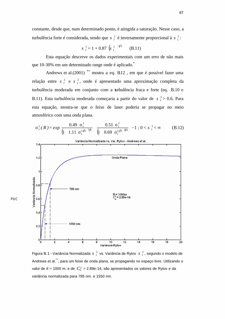
Andrews et al.(2001) ** mostra a eq. B.12 , em que é possível fazer uma

relação entre 2Iσ e 2

1σ , onde é apresentado uma aproximação completa da

turbulência moderada em conjunto com a turbulência fraca e forte (eq. B.10 e

B.11). Esta turbulência moderada começaria a partir do valor de 2Iσ > 0.6. Para

esta equação, mostra-se que o feixe de laser poderia se propagar no meio

atmosférico com uma onda plana.

( ) ( )1

6901

510

1111

49065512

1

21

675121

212 −

σ⋅+

σ⋅+

σ⋅+

σ⋅=σ

.

.

.

.exp)R( I ; 0 < 2

1σ < ∞ (B.12)

Figura B.1 - Variância Normalizada 2Iσ vs. Variância de Rytov 2

1σ , segundo o modelo de

Andrews et al.**, para um feixe de onda plana, se propagando no espaço livre. Utilizando o

valor de R = 1000 m. e de 2nC = 2.89e-14, são apresentados os valores de Rytov e da

variância normalizada para 785 nm. e 1550 nm.

DBD


88

A descrição gráfica da eq. B.12 está apresentada na Figura B.1. Nesta Figura é

indicado que, em uma turbulência fraca haverá maior cintilação em 785 nm; e em

uma turbulência forte a cintilação será maior em 1550 nm. Na Figura 2.12 pode ser

conferido que a variância de Rytov 21σ encontra-se na faixa da turbulência fraca

(1550nm) e moderada (785 nm). Porem, quando é modificado algum valor que

define a variância de Rytov 21σ (comprimento de onda ?, a distancia do range R ou

o valor de 2nC ), a turbulência fraca pode passar para 1550 nm e a forte passaria

para 785 nm, ficando coerente com as equações B.10, B.11 e B.12.

*

ZUEV, V.E., Laser-Light Transmission Through the Atmosphere, Laser Monitoring of the Atmosphere, Editor: E.D.

Hinkley, Topics in Applied Physics - Volume 14, Springer-Verlag, Germany, 1976, Cap3, pág 29-69. ** ANDREWS, L.C., PHILLIPS, R.L., HOPEN, C.Y.; “Laser Beam Scintillation with Applicatio ns”, SPIE PRESS,

Bellingham-Washington USA, May 2001, pag 101.

DBD


89

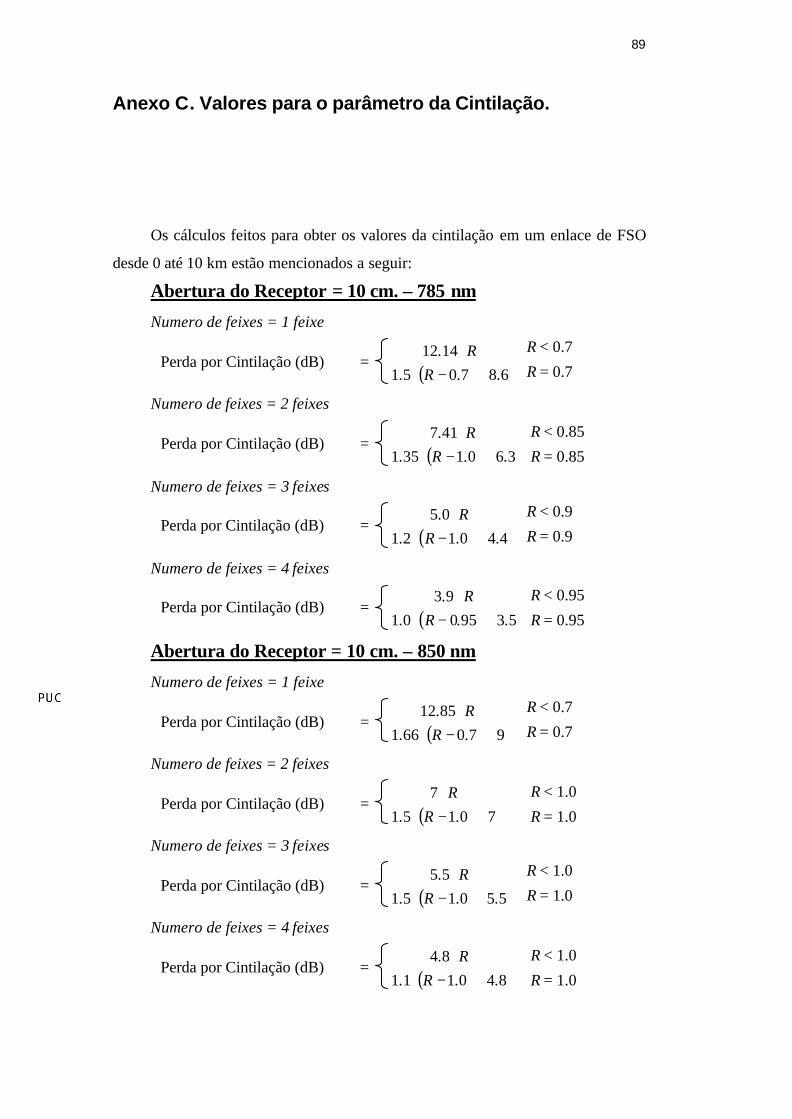
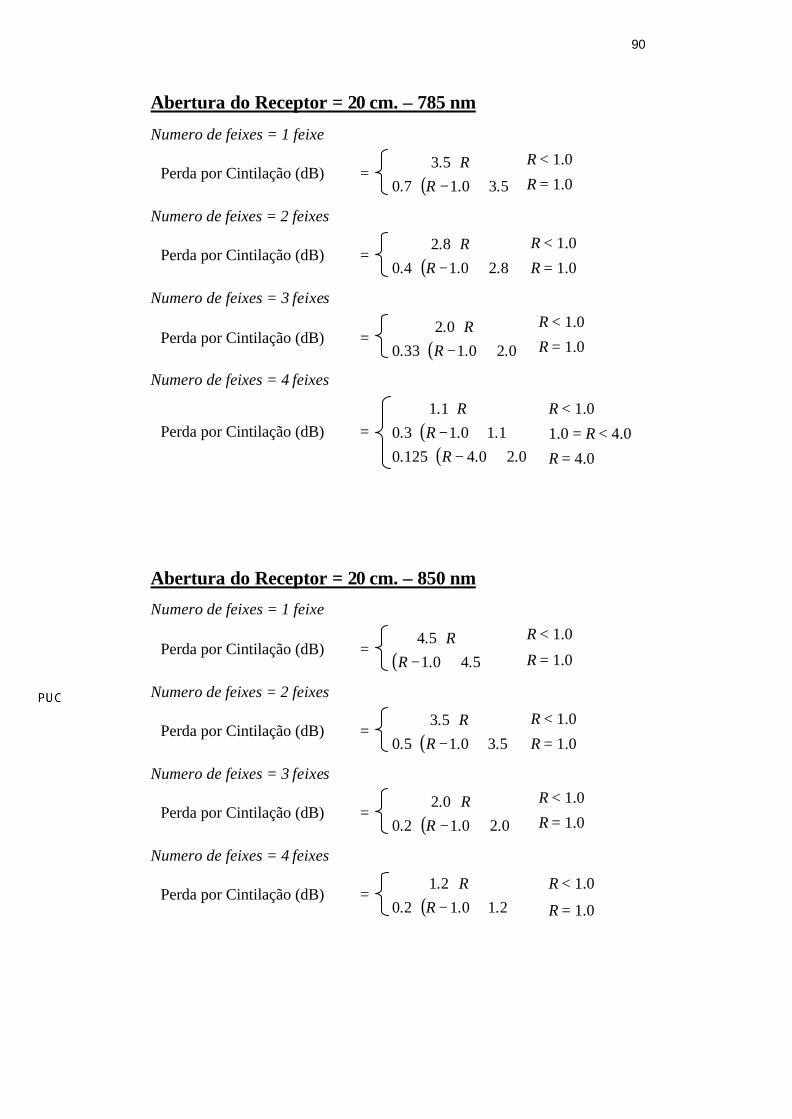
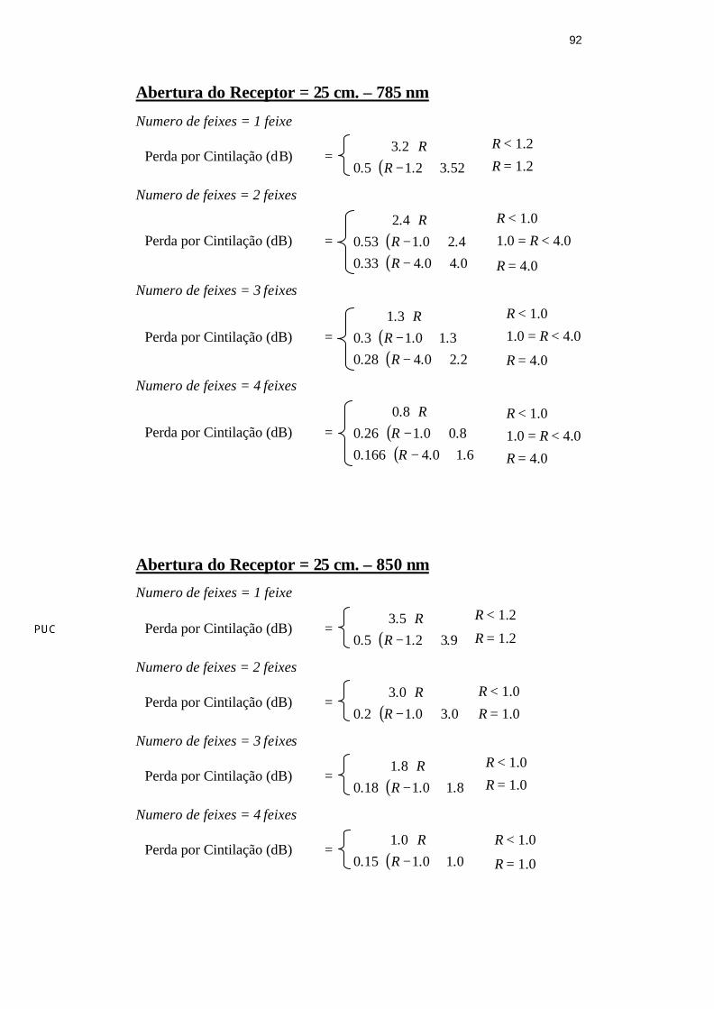
Anexo C. Valores para o parâmetro da Cintilação.

Os cálculos feitos para obter os valores da cintilação em um enlace de FSO

desde 0 até 10 km estão mencionados a seguir:

Abertura do Receptor = 10 cm. – 785 nm

Numero de feixes = 1 feixe

Perda por Cintilação (dB) = ( ) 687051

1412..R.

R.+−⋅

⋅

Numero de feixes = 2 feixes


417..R.

R.+−⋅

⋅



05..R.

R.+−⋅

⋅



93..R.

R.+−⋅

⋅




8512+−⋅

⋅.R.R.



7+−⋅

⋅.R.

R



55..R.

R.+−⋅

⋅



84..R.

R.+−⋅

⋅

R < 0.7

R = 0.7

R < 0.85

R = 0.85

R < 0.9

R = 0.9

R < 0.95

R = 0.95

R < 0.7

R = 0.7

R < 1.0

R = 1.0

R < 1.0

R = 1.0

R < 1.0

R = 1.0

DBD


90




53..R.

R.+−⋅

⋅



82..R.

R.+−⋅

⋅



02..R.

R.+−⋅

⋅


Perda por Cintilação (dB) = ( )( ) 02041250

11013011

..R...R.

R.

+−⋅+−⋅

⋅




54..R

R.+−

⋅



53..R.

R.+−⋅

⋅



02..R.

R.+−⋅

⋅



21..R.

R.+−⋅

⋅

R < 1.0

R = 1.0

R < 1.0

R = 1.0

R < 1.0

R = 1.0

R < 1.0

1.0 = R < 4.0

R = 4.0

R < 1.0

R = 1.0

R < 1.0

R = 1.0

R < 1.0

R = 1.0

R < 1.0

R = 1.0

DBD


91



Perda por Cintilação (dB) = ( )( )( ) 01442651

610218320860334

3313

..R.

..R...R.

R.

+−⋅+−⋅+−⋅

⋅


Perda por Cintilação (dB) = ( )

( )( ) 091241

86214422747005

16

..R...R.

..R.R.

+−⋅+−⋅

+−⋅⋅



052142164

..R...R.

R.

+−⋅+−⋅

⋅


Perda por Cintilação (dB) = ( )( )( ) 41065650

966216159421641

833

..R...R...R.

R.

+−⋅+−⋅+−⋅

⋅

R < 0.6

0.6 = R < 1.2

1.2 = R < 2.4

R = 2.4

R < 0.7

0.7 = R < 1.2

1.2 = R < 2.1

R = 2.1

R < 1.2

1.2 = R < 2.2

R = 2.2

R < 1.2

1.2 = R < 2.6

2.6 = R < 5.6

R = 5.6

R = 1.0

DBD


92




23..R.

R.+−⋅

⋅



420153042

..R...R.

R.

+−⋅+−⋅

⋅



31013031

..R...R.

R.

+−⋅+−⋅

⋅



800126080

..R...R.

R.

+−⋅+−⋅

⋅




53..R.

R.+−⋅

⋅



03..R.

R.+−⋅

⋅



81..R.

R.+−⋅

⋅



01..R.

R.+−⋅

⋅

R < 1.2

R = 1.2

R < 1.0

1.0 = R < 4.0

R = 4.0

R < 1.0

1.0 = R < 4.0

R = 4.0

R < 1.0

1.0 = R < 4.0

R = 4.0

R < 1.2

R = 1.2

R < 1.0

R = 1.0

R < 1.0

R = 1.0

R < 1.0

R = 1.0

DBD


93

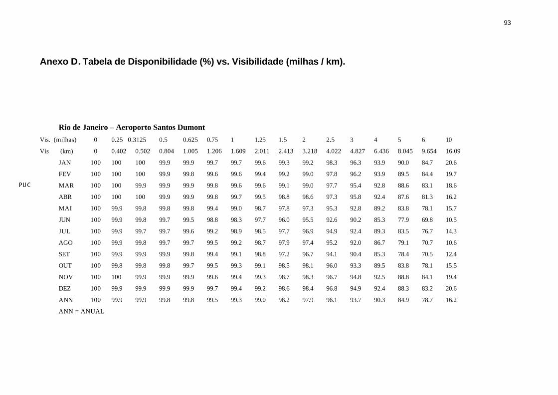
Anexo D. Tabela de Disponibilidade (%) vs. Visibilidade (milhas / km).

Rio de Janeiro – Aeroporto Santos Dumont Vis. (milhas) 0 0.25 0.3125 0.5 0.625 0.75 1 1.25 1.5 2 2.5 3 4 5 6 10

Vis (km) 0 0.402 0.502 0.804 1.005 1.206 1.609 2.011 2.413 3.218 4.022 4.827 6.436 8.045 9.654 16.09

JAN 100 100 100 99.9 99.9 99.7 99.7 99.6 99.3 99.2 98.3 96.3 93.9 90.0 84.7 20.6

FEV 100 100 100 99.9 99.8 99.6 99.6 99.4 99.2 99.0 97.8 96.2 93.9 89.5 84.4 19.7

MAR 100 100 99.9 99.9 99.9 99.8 99.6 99.6 99.1 99.0 97.7 95.4 92.8 88.6 83.1 18.6

ABR 100 100 100 99.9 99.9 99.8 99.7 99.5 98.8 98.6 97.3 95.8 92.4 87.6 81.3 16.2

MAI 100 99.9 99.8 99.8 99.8 99.4 99.0 98.7 97.8 97.3 95.3 92.8 89.2 83.8 78.1 15.7

JUN 100 99.9 99.8 99.7 99.5 98.8 98.3 97.7 96.0 95.5 92.6 90.2 85.3 77.9 69.8 10.5

JUL 100 99.9 99.7 99.7 99.6 99.2 98.9 98.5 97.7 96.9 94.9 92.4 89.3 83.5 76.7 14.3

AGO 100 99.9 99.8 99.7 99.7 99.5 99.2 98.7 97.9 97.4 95.2 92.0 86.7 79.1 70.7 10.6

SET 100 99.9 99.9 99.9 99.8 99.4 99.1 98.8 97.2 96.7 94.1 90.4 85.3 78.4 70.5 12.4

OUT 100 99.8 99.8 99.8 99.7 99.5 99.3 99.1 98.5 98.1 96.0 93.3 89.5 83.8 78.1 15.5

NOV 100 100 99.9 99.9 99.9 99.6 99.4 99.3 98.7 98.3 96.7 94.8 92.5 88.8 84.1 19.4

DEZ 100 99.9 99.9 99.9 99.9 99.7 99.4 99.2 98.6 98.4 96.8 94.9 92.4 88.3 83.2 20.6

ANN 100 99.9 99.9 99.8 99.8 99.5 99.3 99.0 98.2 97.9 96.1 93.7 90.3 84.9 78.7 16.2

ANN = ANUAL

DBD


94

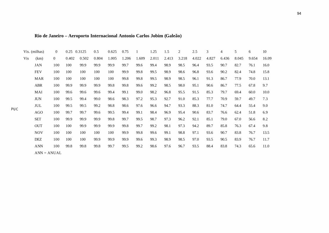
Rio de Janeiro – Aeroporto Internacional Antonio Carlos Jobim (Galeão)

Vis. (milhas) 0 0.25 0.3125 0.5 0.625 0.75 1 1.25 1.5 2 2.5 3 4 5 6 10

Vis (km) 0 0.402 0.502 0.804 1.005 1.206 1.609 2.011 2.413 3.218 4.022 4.827 6.436 8.045 9.654 16.09

JAN 100 100 99.9 99.9 99.9 99.7 99.6 99.4 98.9 98.5 96.4 93.5 90.7 82.7 76.1 16.0

FEV 100 100 100 100 100 99.9 99.8 99.5 98.9 98.6 96.8 93.6 90.2 82.4 74.8 15.8

MAR 100 100 100 100 100 99.8 99.8 99.5 98.9 98.5 96.1 91.3 86.7 77.9 70.0 13.1

ABR 100 99.9 99.9 99.9 99.8 99.8 99.6 99.2 98.5 98.0 95.1 90.6 86.7 77.5 67.8 9.7

MAI 100 99.6 99.6 99.6 99.4 99.1 99.0 98.2 96.8 95.5 91.5 85.3 79.7 69.4 60.0 10.0

JUN 100 99.5 99.4 99.0 98.6 98.3 97.2 95.3 92.7 91.0 85.3 77.7 70.9 59.7 49.7 7.3

JUL 100 99.5 99.5 99.2 98.8 98.6 97.6 96.6 94.7 93.3 88.3 81.0 74.7 64.4 55.4 9.0

AGO 100 99.7 99.7 99.6 99.5 99.4 99.1 98.4 96.9 95.4 90.6 83.7 76.6 62.4 51.8 6.9

SET 100 99.9 99.9 99.9 99.8 99.7 99.5 98.7 97.3 96.2 92.1 85.1 79.0 67.0 56.6 8.2

OUT 100 100 99.9 99.9 99.9 99.8 99.7 99.2 98.1 97.3 94.2 89.7 85.8 76.3 67.4 9.8

NOV 100 100 100 100 100 99.9 99.8 99.6 99.1 98.8 97.1 93.6 90.7 83.8 76.7 13.5

DEZ 100 100 100 99.9 99.9 99.9 99.6 99.3 98.9 98.5 97.0 93.5 90.5 83.9 76.7 11.7

ANN 100 99.8 99.8 99.8 99.7 99.5 99.2 98.6 97.6 96.7 93.5 88.4 83.8 74.3 65.6 11.0

ANN = ANUAL

DBD


95

Anexo E.

CONTRIBUIÇÃO ORIGINAL DO AUTOR

“SIMULATION AND DEVELOPMENT

OF A FSO SYSTEM AT AN URBAN

ENVIRONMENT IN RIO DE JANEIRO”

Vol. 5550-24

SPIE 2004

DENVER, COLORADO

Apresentado em 03 de Agosto de 2004

DBD


96

Simulation and development of a FSO system at an urban environment in Rio de Janeiro

A. Huanachín*, M. Mosso, B. Guedes and A. Podcameni¤.

Catholic University of Rio de Janeiro CETUC / PUC-Rio - R. Marquês de São Vicente, 225, 7K, Gávea

Rio de Janeiro / RJ - 22453-900 – Brazil.

A procedure for the analysis, modeling, and a practical trial of a Free-Space Optics (FSO) system is presented. The procedure has been conducted in the urban area of Rio de Janeiro, in 2002. Firstly, the transmitter and receiver characteristics are considered. Next, three additional parameters are introduced: they are: the atmospheric loss, the geometric loss and the scintillation. In this last parameter, a few ways how scintillation might be expressed in dB and translated into a power balance equation, is presented. Other fixed parameters, dealing with additional losses, are subsequently inserted. The FSO system availability is exhibited, using airports visibility data, leading to a prediction of the systemic availability. Attention is then focused on the Bit Error Rate, BER, which relates with the Recommendation ITU-T G.826. Within this last Recommendation, it is possible to perform a FSO analysis with respect to the climatic variation. The experiment has encompassed some short periods in which this city presents a strong morning fog. It is finally shown that FSO is a competitive and reliable transmission technology, provided proper and correct use. Keywords: FSO, Last mile, BER, Recommendation ITU-T, G.826, SONET, SDH, Optical site in Rio de Janeiro

1. INTRODUCTION Present telecommunication systems use two types of technologies: (a) - Environment confined, as optical fibers or coaxial cables, and, (b) - Free space (non-confined) systems as, for example, Microwaves and/or RF links. Present telecommunication systems use two types of technologies: (a) - Environment confined, as optical fibers or coaxial cables, and, (b) - Free space (non-confined) systems as, for example, Microwaves and/or RF links. Free-Space Optics (FSO) is inserted in the second category, however, it possess some characteristics of the first one. Many of the elements used in FSO are also employed in optical fibers, although the FSO transmission environment; is the air1. The FSO systems are getting popular due to a growing Internet demand. With FSO communications, data transmission, images, sound and video applications may be sent at a few Gigabits for second without the necessity of deploying an optical fiber, and/or digging a trench in someone else’s neighborhood. Briefly, the advantages of an FSO system may be put as: - Fast and cheap installation of the system. - It needs no license to use the electromagnetic spectrum. - It launches a competitive and broadband link; similar to the optical fiber, and much broader than the one used in microwave radios. - FSO does not cause electromagnetic interference. Disadvantages found in an FSO system are related with the optical propagation across the atmosphere. The wavelengths are comparable in size with several environmental particles and molecules. The laser beam energy may be absorbed or scattered by these particles. This phenomenon will be addressed ahead. The most used wavelengths for FSO are the 785, 850 and the 1550 nm waves. This sort of preference is because components for these wavelengths are commercially and widely available for optical fibers applications2. In the specific ¤ [email protected]; phone 55 21 3114-1685; fax 55 21 3114-1154 www.cetuc.puc-rio.br * [email protected]

DBD


97

case of a 1550 nm apparatus, FSO may easily use multi-wavelength beam, supported by DWDM technology3. 1.1 Impairments The three conditions more significant which affect the FSO link are: - Absorption. - Scattering. - Scintillation. These three conditions attenuate the received power, affecting the availability of the link4. The optical wireless systems presents low cost and rapidity in their installation. They may be installed in the same structure of a cellular net site, circumventing interference with microwave systems. Additionally, the acceptance test period is reduced from months to only a couple of days. For the FSO design procedure is important to reach a basic FSO equation4. Consequently, diverse parameters will be hereupon introduced. 1.2 Transmitter and receiver The transmitted and received powers are defined in Watts (W). PTX = emitted power by the transmitter. PRX = minimum power arriving into the receiver, for a distance R. 1.3 Atmospheric loss The law that conducts the attenuation of the laser radiation in the atmosphere is the Beer´s law.

LAtm = Re σ− (1) where: σ = attenuation coefficient R = transmission length of the laser Attenuation coefficient σ depends of the visibility and the wavelength λ :

q

nmV

−

=

55091.3 λσ (2)

where: V = Visibility (km) λ = Wavelength (nm)

q =

1.6 for V > 50 km ; 1.3 for 6 < V < 50 km ; 0.585 V -1/3 for V < 6 km 4.

1.4 Geometric loss Geometric loss depends very much of the received power after to have crossed the free space, and also of both the transmitter and receiver area, as shown in Figure 4.

LGeo ( )2R

4 SA*N

SA

T

R

⋅θπ

+= (3)

where: SAR = Receiver surface (m2) SAT = Transmitter surface (m2) θ = Beam divergence area (mrad) R = Transmission length of the laser N = Number of transmitters used. This is a new contribution for geometric loss. If SAT is very small, it can to be omitted4. 1.5 Scintillation loss Scintillation is defined as a temporal and spatial light intensity variation, caused by atmospheric turbulence that cross the FSO link. Atmospheric turbulence is originated by temperature, pression or winds that movies between the ground

DBD


98

and the air. From those variations, are created air hot bubbles which distort the laser path.

Rytov´s variance 21σ is used to simplify the scintillation parameter5:

LScint = 611

6722

1 23.1 RkC n=σ (4) where:

21σ = Rytov´s variance. 2nC = Refractive Index Structure Parameter

k = wavenumber = λπ /2 R = length of the link (meters) Rytov´s variance 2

1σ represent the normalized variance of the irradiance which will increase or will diminish in

accordance with the value of 2nC . Irradiance is the incident power on a surface. Unit is measured in W/m2.

2nC will define if the atmospheric turbulence is weak, moderate or strong: 6

( ) ( )( )( )

2

26

32

2

2

)(

)(1080

,,)(

×

+−= −

zT

zP

r

zrxTzxTzC n (5)

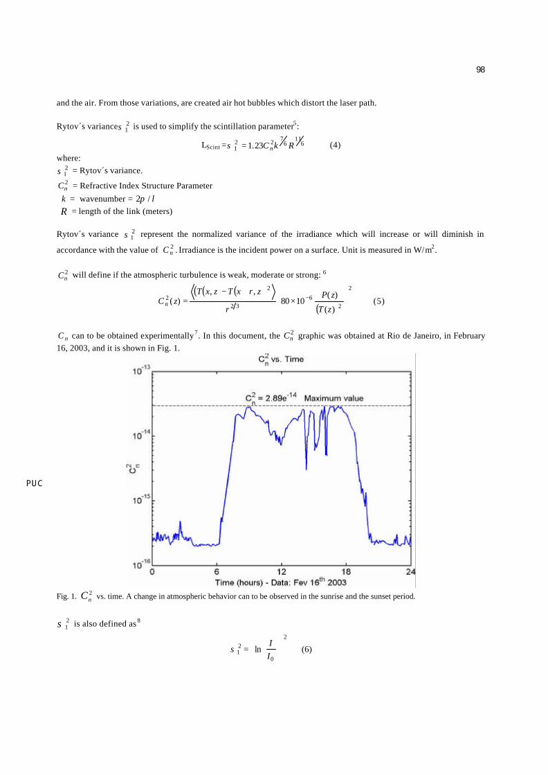
nC can to be obtained experimentally7. In this document, the 2nC graphic was obtained at Rio de Janeiro, in February

16, 2003, and it is shown in Fig. 1.

Fig. 1. 2

nC vs. time. A change in atmospheric behavior can to be observed in the sunrise and the sunset period.

21σ is also defined as 8

2

0

21 ln

=

II

σ (6)

DBD


99

Equation (6) defines: I = Instantaneous irradiance which arrives at the receiver. 0I = Middle Irradiance received. In order to reach above value, written in dB9,10 equation (7) is next presented:

LScint =

0 log 10

II

dB (7)

Equations (6) and (7) will allow for determining the scintillation loss. For illustration, a value of 21σ = 1.3, will yield a

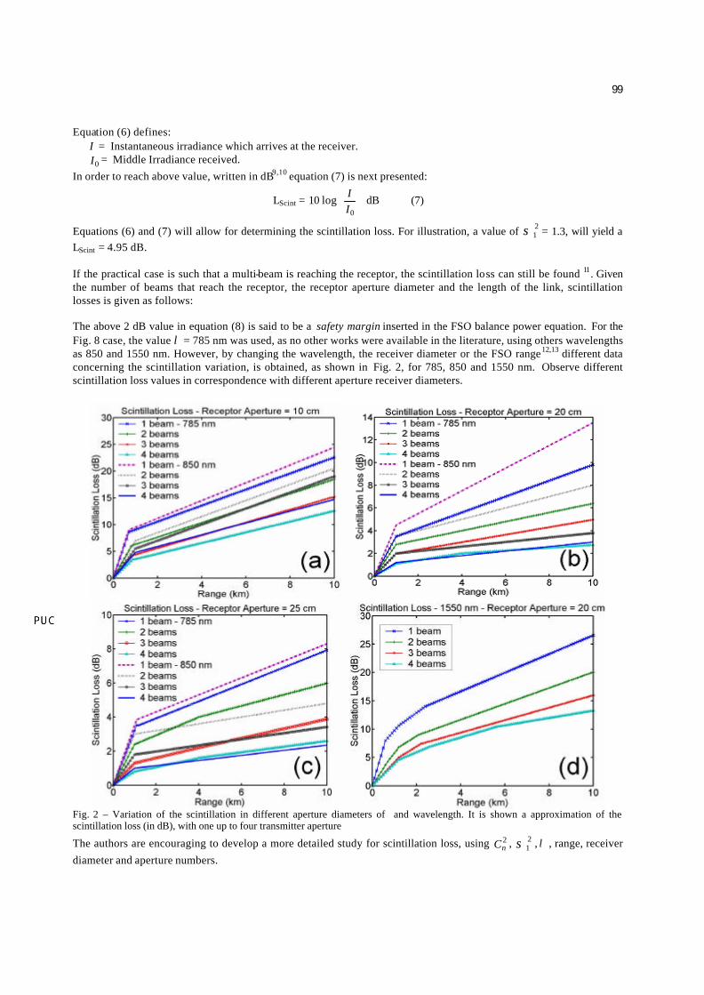
LScint = 4.95 dB. If the practical case is such that a multi-beam is reaching the receptor, the scintillation loss can still be found 11. Given the number of beams that reach the receptor, the receptor aperture diameter and the length of the link, scintillation losses is given as follows: The above 2 dB value in equation (8) is said to be a safety margin inserted in the FSO balance power equation. For the Fig. 8 case, the value λ = 785 nm was used, as no other works were available in the literature, using others wavelengths as 850 and 1550 nm. However, by changing the wavelength, the receiver diameter or the FSO range12,13 different data concerning the scintillation variation, is obtained, as shown in Fig. 2, for 785, 850 and 1550 nm. Observe different scintillation loss values in correspondence with different aperture receiver diameters.

Fig. 2 – Variation of the scintillation in different aperture diameters of and wavelength. It is shown a approximation of the scintillation loss (in dB), with one up to four transmitter aperture

The authors are encouraging to develop a more detailed study for scintillation loss, using 2nC , 2

1σ , λ , range, receiver diameter and aperture numbers.

DBD


100

1.6 Others Loss in the FSO link FSO link presents other inherents losses. It is additionally recommended 4 to use typical correcting factors: - Mispoint losses: LMisp = 3 dB e - Optical losses in the receiver: LRXOp = 9 dB.

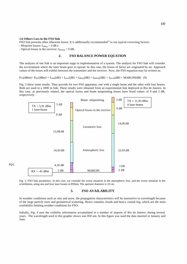
2. FSO BALANCE POWER EQUATION The analysis of one link is an important stage in implementation of a system. The analysis for FSO link will consider the environment where the laser beam goes to spread. In this case, the losses of factor are originated by air. Approach values of the losses will exhibit between the transmitter and the receiver. Now, the FSO equation may be written as: PTX[dBm]= PRX[dBm] + LAtm[dB] + LGeo[dB] + LMisp[dB] + LRXOp[dB] + LScint[dB] + MARGIN[dB] (9) Fig. 3 show some results. They provide for two FSO apparatus; one with a single beam and the other with four beams. Both are used in a 1000 m link. These results were obtained from an experimental link deployed in Rio de Janeiro. In this case, as previously related, the optical losses and beam mispointing losses have fixed values of 9 and 3 dB, respectively.

Fig. 3. FSO link parameters. In this case, we consider the worse situation in the atmospheric loss, and the worse situation in the scintillation, using one and four laser beams in 850nm. The aperture diameter is 10 cm.

3. FSO AVAILABILITY In weather conditions such as rain and snow, the propagation characteristics will be insensitive to wavelength because of the large particle sizes and geometrical scattering. Heavy cumulus clouds and heavy coastal fog, which are the main availability limiting weather conditions for FSO. Initially, Fig. 4 uses the visibility information accumulated in a number of airports of Rio de Janeiro, during several years. The wavelength used in this graphic shows was 850 nm. In this figure was used the data inserted in January and June.

TX = 5,91 dBm 1 laser beam

RX = -41 dBm MARGIN

Beam mispointing

Optical losses in the receiver

Geometric loss

Atmospheric loss

3 dB

9 dB

13,98 dB

14,43 dB

4,50 dB

2 dB

TX = 11,93 dBm 4 laser beams

3 dB

9 dB

14,00 dB

23,93 dB

1 d B 2 dB

DBD


101

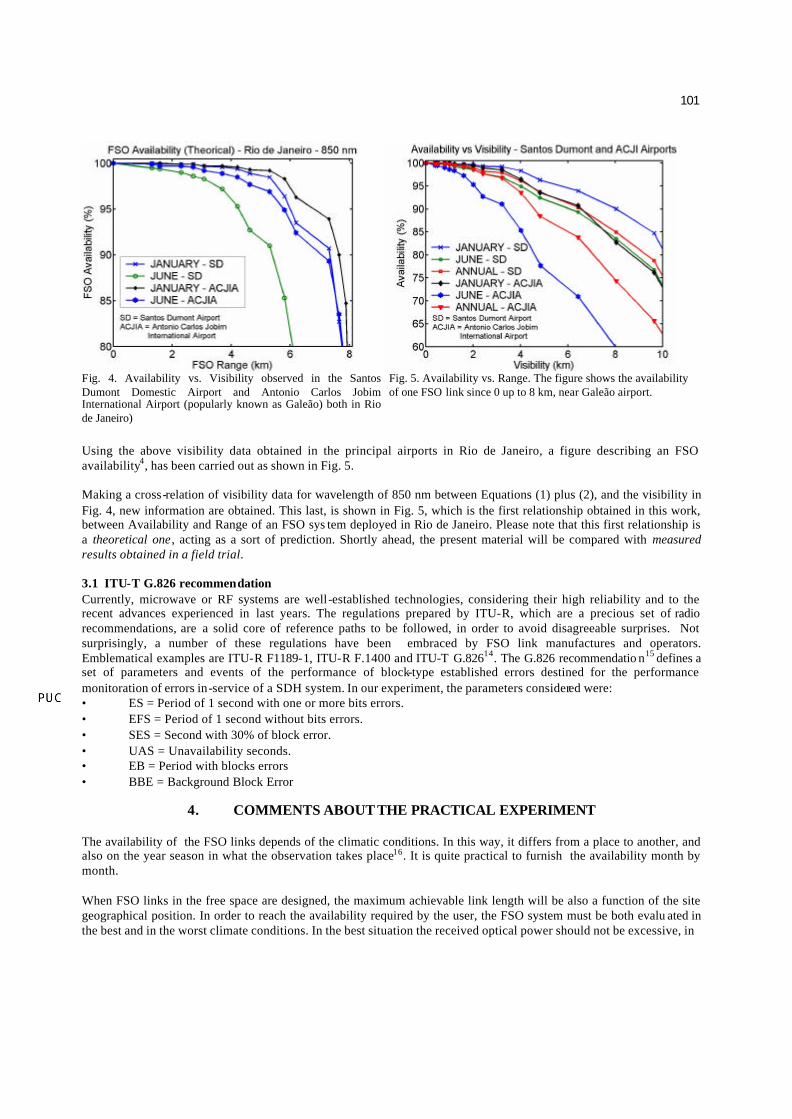
Fig. 4. Availability vs. Visibility observed in the Santos Dumont Domestic Airport and Antonio Carlos Jobim International Airport (popularly known as Galeão) both in Rio de Janeiro)

Fig. 5. Availability vs. Range. The figure shows the availability of one FSO link since 0 up to 8 km, near Galeão airport.

Using the above visibility data obtained in the principal airports in Rio de Janeiro, a figure describing an FSO availability4, has been carried out as shown in Fig. 5. Making a cross-relation of visibility data for wavelength of 850 nm between Equations (1) plus (2), and the visibility in Fig. 4, new information are obtained. This last, is shown in Fig. 5, which is the first relationship obtained in this work, between Availability and Range of an FSO sys tem deployed in Rio de Janeiro. Please note that this first relationship is a theoretical one , acting as a sort of prediction. Shortly ahead, the present material will be compared with measured results obtained in a field trial. 3.1 ITU-T G.826 recommendation Currently, microwave or RF systems are well-established technologies, considering their high reliability and to the recent advances experienced in last years. The regulations prepared by ITU-R, which are a precious set of radio recommendations, are a solid core of reference paths to be followed, in order to avoid disagreeable surprises. Not surprisingly, a number of these regulations have been embraced by FSO link manufactures and operators. Emblematical examples are ITU-R F1189-1, ITU-R F.1400 and ITU-T G.82614. The G.826 recommendatio n15 defines a set of parameters and events of the performance of block-type established errors destined for the performance monitoration of errors in-service of a SDH system. In our experiment, the parameters considered were: • ES = Period of 1 second with one or more bits errors. • EFS = Period of 1 second without bits errors. • SES = Second with 30% of block error. • UAS = Unavailability seconds. • EB = Period with blocks errors • BBE = Background Block Error

4. COMMENTS ABOUT THE PRACTICAL EXPERIMENT The availability of the FSO links depends of the climatic conditions. In this way, it differs from a place to another, and also on the year season in what the observation takes place16. It is quite practical to furnish the availability month by month. When FSO links in the free space are designed, the maximum achievable link length will be also a function of the site geographical position. In order to reach the availability required by the user, the FSO system must be both evalu ated in the best and in the worst climate conditions. In the best situation the received optical power should not be excessive, in

DBD


102

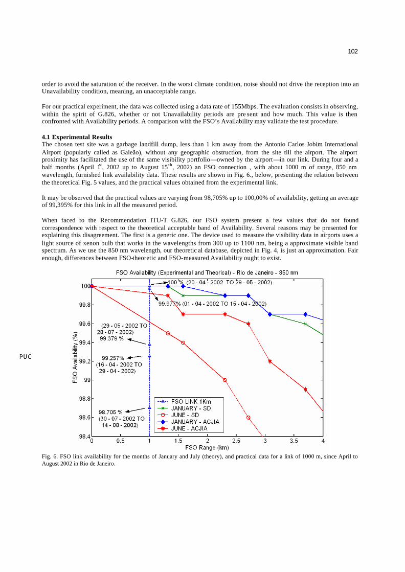
order to avoid the saturation of the receiver. In the worst climate condition, noise should not drive the reception into an Unavailability condition, meaning, an unacceptable range. For our practical experiment, the data was collected using a data rate of 155Mbps. The evaluation consists in observing, within the spirit of G.826, whether or not Unavailability periods are pre sent and how much. This value is then confronted with Availability periods. A comparison with the FSO’s Availability may validate the test procedure. 4.1 Experimental Results The chosen test site was a garbage landfill dump, less than 1 km away from the Antonio Carlos Jobim International Airport (popularly called as Galeão), without any geographic obstruction, from the site till the airport. The airport proximity has facilitated the use of the same visibility portfolio—owned by the airport—in our link. During four and a half months (April 1st, 2002 up to August 15 th, 2002) an FSO connection , with about 1000 m of range, 850 nm wavelength, furnished link availability data. These results are shown in Fig. 6., below, presenting the relation between the theoretical Fig. 5 values, and the practical values obtained from the experimental link. It may be observed that the practical values are varying from 98,705% up to 100,00% of availability, getting an average of 99,395% for this link in all the measured period. When faced to the Recommendation ITU-T G.826, our FSO system present a few values that do not found correspondence with respect to the theoretical acceptable band of Availability. Several reasons may be presented for explaining this disagreement. The first is a generic one. The device used to measure the visibility data in airports uses a light source of xenon bulb that works in the wavelengths from 300 up to 1100 nm, being a approximate visible band spectrum. As we use the 850 nm wavelength, our theoretic al database, depicted in Fig. 4, is just an approximation. Fair enough, differences between FSO-theoretic and FSO-measured Availability ought to exist.

Fig. 6. FSO link availability for the months of January and July (theory), and practical data for a link of 1000 m, since April to August 2002 in Rio de Janeiro.

DBD


103

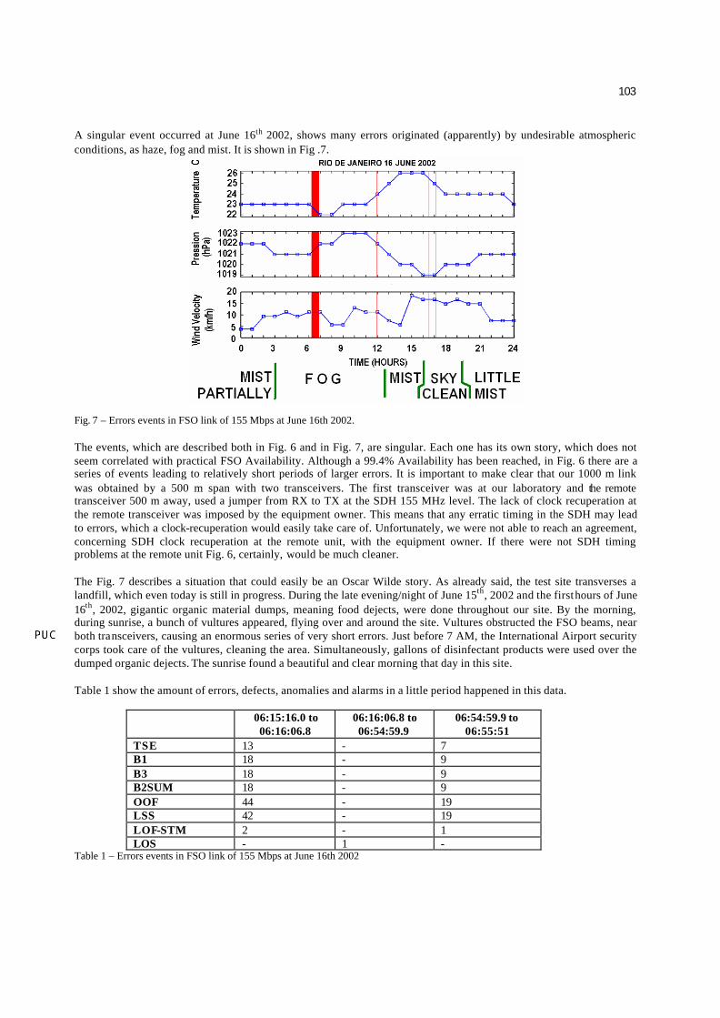
A singular event occurred at June 16th 2002, shows many errors originated (apparently) by undesirable atmospheric conditions, as haze, fog and mist. It is shown in Fig .7.

Fig. 7 – Errors events in FSO link of 155 Mbps at June 16th 2002. The events, which are described both in Fig. 6 and in Fig. 7, are singular. Each one has its own story, which does not seem correlated with practical FSO Availability. Although a 99.4% Availability has been reached, in Fig. 6 there are a series of events leading to relatively short periods of larger errors. It is important to make clear that our 1000 m link was obtained by a 500 m span with two transceivers. The first transceiver was at our laboratory and the remote transceiver 500 m away, used a jumper from RX to TX at the SDH 155 MHz level. The lack of clock recuperation at the remote transceiver was imposed by the equipment owner. This means that any erratic timing in the SDH may lead to errors, which a clock-recuperation would easily take care of. Unfortunately, we were not able to reach an agreement, concerning SDH clock recuperation at the remote unit, with the equipment owner. If there were not SDH timing problems at the remote unit Fig. 6, certainly, would be much cleaner. The Fig. 7 describes a situation that could easily be an Oscar Wilde story. As already said, the test site transverses a landfill, which even today is still in progress. During the late evening/night of June 15th, 2002 and the first hours of June 16th, 2002, gigantic organic material dumps, meaning food dejects, were done throughout our site. By the morning, during sunrise, a bunch of vultures appeared, flying over and around the site. Vultures obstructed the FSO beams, near both transceivers, causing an enormous series of very short errors. Just before 7 AM, the International Airport security corps took care of the vultures, cleaning the area. Simultaneously, gallons of disinfectant products were used over the dumped organic dejects. The sunrise found a beautiful and clear morning that day in this site. Table 1 show the amount of errors, defects, anomalies and alarms in a little period happened in this data.

06:15:16.0 to 06:16:06.8

06:16:06.8 to 06:54:59.9

06:54:59.9 to 06:55:51

TSE 13 - 7 B1 18 - 9 B3 18 - 9 B2SUM 18 - 9 OOF 44 - 19 LSS 42 - 19 LOF-STM 2 - 1 LOS - 1 -

Table 1 – Errors events in FSO link of 155 Mbps at June 16th 2002

DBD


104

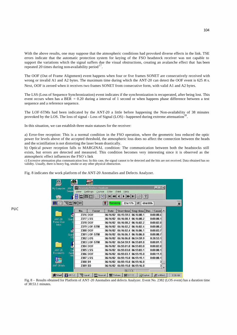
With the above results, one may suppose that the atmospheric conditions had provoked diverse effects in the link. TSE errors indicate that the automatic protection system for keying of the FSO headstock receiver was not capable to support the variations which the signal suffers due the visual obstructions, creating an avalanche effect that has been repeated 20 times during non-availability period17. The OOF (Out of Frame Alignment) event happens when four or five frames SONET are consecutively received with wrong or invalid A1 and A2 bytes. The maximum time during which the ANT-20 can detect the OOF event is 625 µ s. Next, OOF is zeroed when it receives two frames SONET from consecutive form, with valid A1 and A2 bytes. The LSS (Loss of Sequence Synchronization) event indicates if the synchronization is recuperated, after being lost. This event occurs when has a BER = 0.20 during a interval of 1 second or when happens phase difference between a test sequence and a reference sequence. The LOF-STMs had been indicated by the ANT-20 a little before happening the Non-availability of 38 minutes provoked by the LOS. The loss of signal - Loss of Signal (LOS) - happened during extreme attenuation18. In this situation, we can establish three main statuses for the receiver: a) Error-free reception: This is a normal condition in the FSO operation, where the geometric loss reduced the optic power for levels above of the accepted threshold, the atmospheric loss does no affect the connection between the heads and the scintillation is not distorting the laser beam drastically. b) Optical power reception falls to MARGINAL condition: The communication between both the headstocks still exists, but errors are detected and measured. This condition becomes very interesting since it is observed as the atmospheric effect influences the FSO´s link c) Excessive attenuation plus communication loss: In this case, the signal cannot to be detected and the bits are not received. Data obtained has no validity. Usually, there is heavy fog, smoke or any other physical obstruction. Fig. 8 indicates the work platform of the ANT-20 Anomalies and Defects Analyzer.

Fig. 8 – Results obtained for Platform of ANT-20 Anomalies and defects Analyzer. Event No. 2382 (LOS event) has a duration time of 38:53.1 minutes.

DBD


105

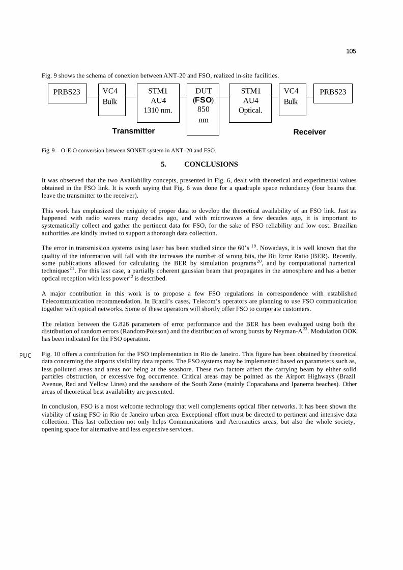
Fig. 9 shows the schema of conexion between ANT-20 and FSO, realized in-site facilities.

Fig. 9 – O-E-O conversion between SONET system in ANT -20 and FSO.

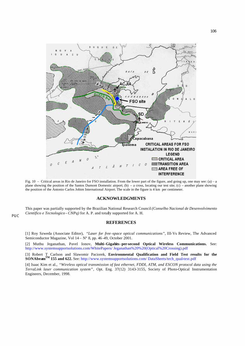
5. CONCLUSIONS It was observed that the two Availability concepts, presented in Fig. 6, dealt with theoretical and experimental values obtained in the FSO link. It is worth saying that Fig. 6 was done for a quadruple space redundancy (four beams that leave the transmitter to the receiver). This work has emphasized the exiguity of proper data to develop the theoretical availability of an FSO link. Just as happened with radio waves many decades ago, and with microwaves a few decades ago, it is important to systematically collect and gather the pertinent data for FSO, for the sake of FSO reliability and low cost. Brazilian authorities are kindly invited to support a thorough data collection. The error in transmission systems using laser has been studied since the 60’s 19. Nowadays, it is well known that the quality of the information will fall with the increases the number of wrong bits, the Bit Error Ratio (BER). Recently, some publications allowed for calculating the BER by simulation programs20, and by computational numerical techniques21. For this last case, a partially coherent gaussian beam that propagates in the atmosphere and has a better optical reception with less power22 is described. A major contribution in this work is to propose a few FSO regulations in correspondence with established Telecommunication recommendation. In Brazil’s cases, Telecom’s operators are planning to use FSO communication together with optical networks. Some of these operators will shortly offer FSO to corporate customers. The relation between the G.826 parameters of error performance and the BER has been evaluated using both the distribution of random errors (Random-Poisson) and the distribution of wrong bursts by Neyman-A23. Modulation OOK has been indicated for the FSO operation. Fig. 10 offers a contribution for the FSO implementation in Rio de Janeiro. This figure has been obtained by theoretical data concerning the airports visibility data reports. The FSO systems may be implemented based on parameters such as, less polluted areas and areas not being at the seashore. These two factors affect the carrying beam by either solid particles obstruction, or excessive fog occurrence. Critical areas may be pointed as the Airport Highways (Brazil Avenue, Red and Yellow Lines) and the seashore of the South Zone (mainly Copacabana and Ipanema beaches). Other areas of theoretical best availability are presented. In conclusion, FSO is a most welcome technology that well complements optical fiber networks. It has been shown the viability of using FSO in Rio de Janeiro urban area. Exceptional effort must be directed to pertinent and intensive data collection. This last collection not only helps Communications and Aeronautics areas, but also the whole society, opening space for alternative and less expensive services.

PRBS23 VC4 Bulk

STM1 AU4

1310 nm.

DUT (FSO)

850 nm

PRBS23 VC4 Bulk

STM1 AU4

Optical.

Transmitter Receiver

DBD


106

Fig. 10 – Critical areas in Rio de Janeiro for FSO installation. From the lower part of the figure, and going up, one may see: (a) – a plane showing the position of the Santos Dumont Domestic airport; (b) – a cross, locating our test site; (c) – another plane showing the position of the Antonio Carlos Jobim International Airport. The scale in the figure is 4 km per centimeter.

ACKNOWLEDGMENTS This paper was partially supported by the Brazilian National Research Council (Conselho Nacional de Desenvolvimento Cientifico e Tecnologico - CNPq) for A. P. and totally supported for A. H.

REFERENCES

[1] Roy Szweda (Associate Editor), “Laser for free -space optical communications”, III-Vs Review, The Advanced Semiconductor Magazine, Vol 14 – N° 8, pp. 46 -49, October 2001. [2] Muthu Jeganathan, Pavel Ionov, Multi-Gigabits -per-second Optical Wireless Communications. See: http://www.systemsupportsolutions.com/WhitePapers/ Jeganathan%20%20(Optical%20Crossing).pdf

[3] Robert T Carlson and Slawomir Paciorek, Environmental Qualification and Field Test results for the SONAbeamTM 155 and 622. See: http://www.systemsupportsolutions.com/ DataSheets/tech_qual-test.pdf [4] Isaac Kim et al., “Wireless optical transmission of fast ethernet, FDDI, ATM, and ESCON protocol data using the TerraLink laser communication system” , Opt. Eng. 37(12) 3143-3155, Society of Photo-Optical Instrumentation Engineers, December, 1998.

DBD


107

[5] L.C. Andrews, R.L. Phillips, C.Y. Hopen, “Laser Beam Scintillation with Applications”, SPIE PRESS, Bellingham-Washington USA, May 2001. [6] L.J. Sanchez et al, “Efficiency of off-axis astronomical adaptative systems: comparison of experimental data for different astronomical sites”, Adaptive Optics System Technologies, SPIE Proc. 4007, Munich, Ed. P.L. Wizinowich, pp. 749 – 755, 2000. [7] S.F. Clifford, ”The Classical Theory of Wave Propagation in a Turbulent Medium”, Laser Beam Propagation in the Atmosphere, Topics in Applied Physics, Vol. 25, pp. 9-43, Editor: J.W. Strohbehn, Springer-Verlag, Berlin-Germany, 1978. [8] TatarskI, Valerian Ilich; Wave propagation in a turbulent medium, New York : Dover Publ., 1967. xiv,if.,285p.,7f. Dover books on physics and mathematical physics. Note: this Dover Publication edition is a reprint of an English Language Translation, previously published in 1961 by McGraw-Hill Book Company (see chapter 12). [9] Yura, H.T.; McKinley, W.G. Optical scintillation statistics for IR ground-to-space laser communication systems , Applied Optics 22, 3353-3358 (1983). [10] Belmonte, A. et al.; Atmospheric-turbulence-induced power-fade statistics for a multiaperture optical receiver , Applied Optics 36, 8632-8638 (1997). [11] Korevaar, Eric et al.; Atmospheric Propagation Characteristics of Highest Importance to Commercial Free Space Optics . See: http://www.mrv.com/library/library.php?ctl=MRV-WP-FSOAtmosProp. [12] I.I. Kim et al.; Measurement of scintillation and link margin for the TerraLink laser communication system, Wireless Technologies and System: Millimeter Wave and Optical, Proc. SPIE, Vol. 3232, 1997, pp 100-118. [13] Harboe, P.B.; Souza, J.R.; Sistemas Ópticos no Espaço Livre: Estudo da Viabilidade de Implementação em Cidade Brasileiras; in: Proceedings of the XX Brazilian Telecommunications Symposium – SBT´03, Oct. 2003 (Rio de Janeiro), pp. 05-08. IEEE Sponsored Meeting.

[14] Wilcock, Duncan; Optical Power Margin or Fade Margin, See: http://www.essentia.it/documenti/WP_Articoli_Tecnici/OPTICAL_POWER_MARGIN_OR_FADE_MARGIN.pdf [15] ITU-T Recommendation G.826, ”Error performance parameters and objectives for intern ational, constant bit rate digital paths at or above the primary rate”, 15 February 1999 [16] Carlson, Robert T.; Reliability and availability in free-space optical systems, Optics in Information Systems – Optical Wireless Communications Edited by Nabeel Riza, October 2001, vol. 12 No 2 page 5 [17] Hischinger, Jochen; Miller, Wolfgang; Synchronization- Jitter- Wander: Basic principles and test equipment , Application Note 71, Wandel & Goltermann GmbH & Co. Printed in Germany. 31pages. [18] TEKTRONIX - Synchronous Optical Network (SONET). See: http://www.iec.org/cgi-bin/acrobat.pl?filecode=131

[19] D. Sette, B. Daino; “Transmission. of Information with Laser Beams”. Laser And Their Applications, Editor: A. Sona, Gordon & Breach, New York, 1976, page 415-439 [20] G. Hansel, E. Kube, J. Becker, J. Haase, P. Schwarz, “Simulation in the Design Process of Free Space Optical Transmission Systems”, Proc. 6th Workshop “Optics in Computing Technology”, pp 45-53 , Paderborn ,Germany, April 3, 2001. [21] J.C. Ricklin, “Free -Space Laser Communication Using a Partially Coherent Source Beam” , Doctoral Dissertation, The John Hopkins University, Baltimore, Maryland, 2002. [22] O.Korotkova, L.C. Andrews, R.L. Phillips, “Phase Diffuser at the Transmitter for Lasercom Link: Effect of Partially Coherent Beam on the Bit-Error Rate.” Proc. SPIE 2003 (submitted). [23] Gloria Patricia Gallo Bedoya, “Análise dos parâmetros de desempenho da recomendação G.826 e sua aplicação ao dimensionamento de enlaces”, Master of Science Dissertation at the Catholic University of Rio de Janeiro, Feb. 28th, 1996, Rio de Janeiro. See: author’s address at the same University.

DBD


Documents

0124852 2005 postextual - DBD PUC RIO€¦ · 77 . scintillation for free-space laser communication at 785 nm and 1550 nm. Proc. Of SPIE Reprint, Vol 3850, 22 Sept 1999, Boston -