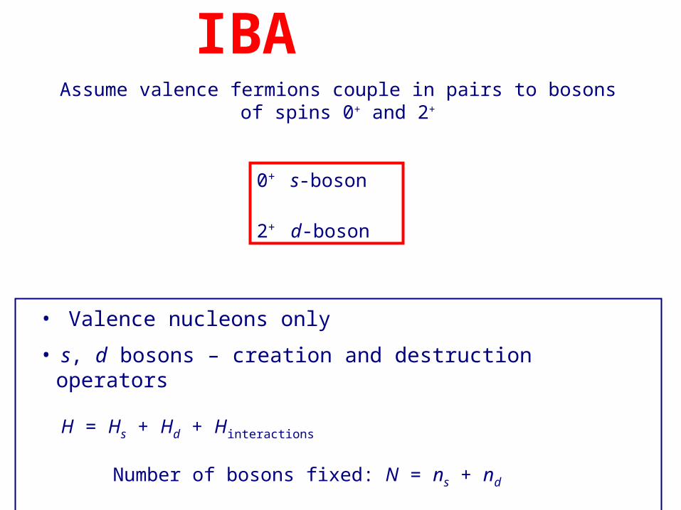
0+ s-boson

2+ d-boson

• Valence nucleons only

• s, d bosons – creation and destruction operators

H = Hs + Hd + Hinteractions

Number of bosons fixed: N = ns + nd

= ½ # of val. protons + ½ # val. neutrons

IBA

Assume valence fermions couple in pairs to bosons of spins 0+ and 2+

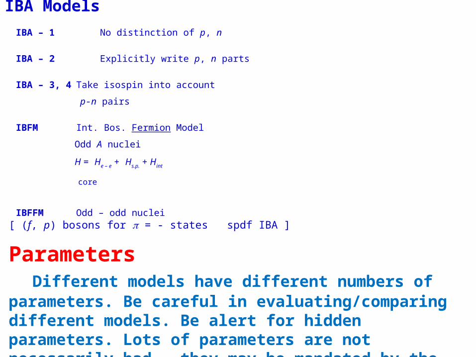
IBA Models

IBA – 1 No distinction of p, n

IBA – 2 Explicitly write p, n parts

IBA – 3, 4 Take isospin into account

p-n pairs

IBFM Int. Bos. Fermion Model

Odd A nuclei

H = He – e + Hs.p. + Hint

core

IBFFM Odd – odd nuclei[ (f, p) bosons for = - states spdf IBA ]

ParametersDifferent models have different numbers of parameters. Be

careful in evaluating/comparing different models. Be alert for hidden parameters. Lots of parameters are not necessarily bad – they may be mandated by the data, but look at them with your eyes open.

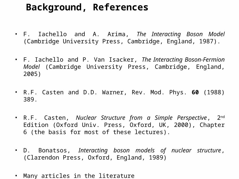
• F. Iachello and A. Arima, The Interacting Boson Model (Cambridge University Press, Cambridge, England, 1987).

• F. Iachello and P. Van Isacker, The Interacting Boson-Fermion Model (Cambridge University Press, Cambridge, England, 2005)

• R.F. Casten and D.D. Warner, Rev. Mod. Phys. 60 (1988) 389.

• R.F. Casten, Nuclear Structure from a Simple Perspective, 2nd Edition (Oxford Univ. Press, Oxford, UK, 2000), Chapter 6 (the basis for most of these lectures).

• D. Bonatsos, Interacting boson models of nuclear structure, (Clarendon Press, Oxford, England, 1989)

• Many articles in the literature

Background, References

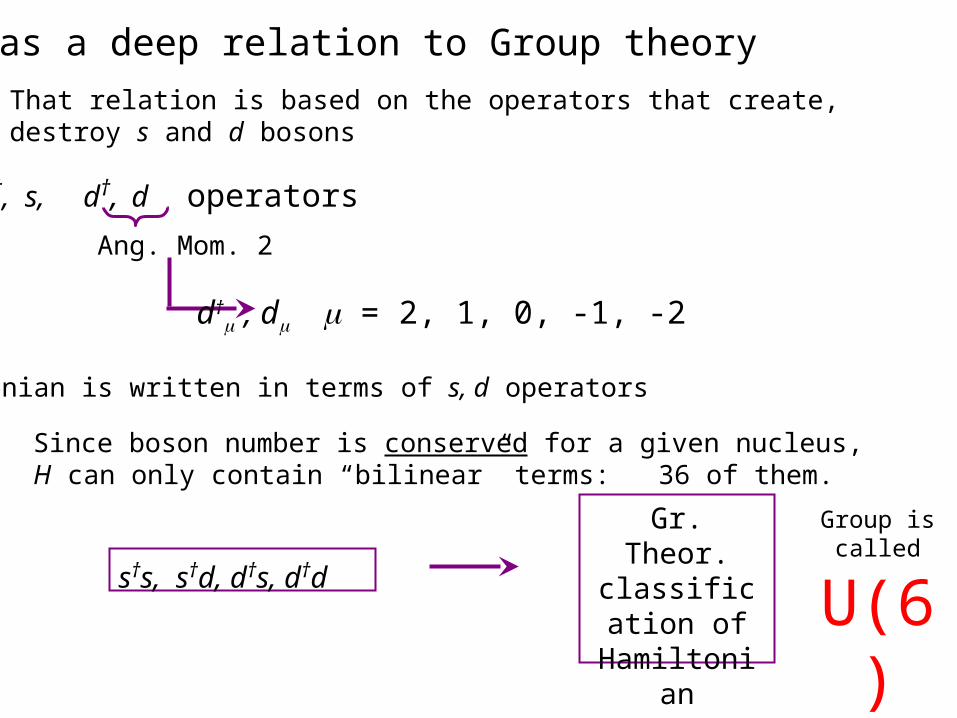
That relation is based on the operators that create, destroy s and d bosons

s†, s, d†, d operators Ang. Mom. 2

d† , d = 2, 1, 0, -1, -2

Hamiltonian is written in terms of s, d operators

Since boson number is conserved for a given nucleus, H can only contain “bilinear” terms: 36 of them.

s†s, s†d, d†s, d†d

Gr. Theor. classification

of Hamiltonian

IBA has a deep relation to Group theory

Group is called

U(6)

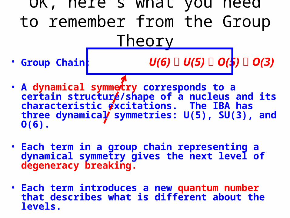
OK, here’s what you need to remember from the Group Theory

• Group Chain: U(6) U(5) O(5) O(3)

• A dynamical symmetry corresponds to a certain structure/shape of a nucleus and its characteristic excitations. The IBA has three dynamical symmetries: U(5), SU(3), and O(6).

• Each term in a group chain representing a dynamical symmetry gives the next level of degeneracy breaking.

• Each term introduces a new quantum number that describes what is different about the levels.

• These quantum numbers then appear in the expression for the energies, in selection rules for transitions, and in the magnitudes of transition rates.

Concept of a Dynamical Symmetry

N

OK, here’s the key point :

Spectrum generating algebra !!

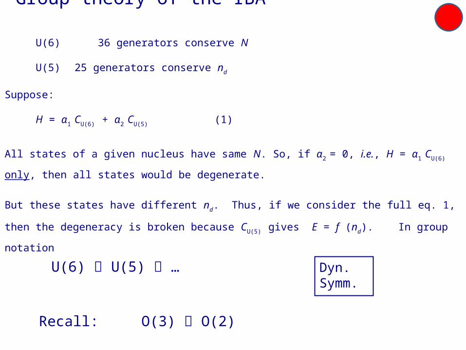
Group theory of the IBA

U(6) 36 generators conserve N

U(5) 25 generators conserve nd

Suppose:

H = α1 CU(6) + α2 CU(5) (1)

All states of a given nucleus have same N. So, if α2 = 0, i.e., H = α1 CU(6) only, then all states would be

degenerate.

But these states have different nd. Thus, if we consider the full eq. 1, then the degeneracy is broken because

CU(5) gives E = f (nd). In group notation

Dyn.Symm.

U(6) U(5) …

Recall: O(3) O(2)

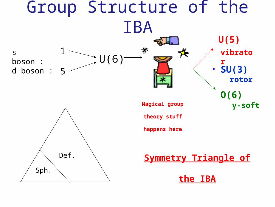
Group Structure of the IBA

s boson :

d boson :

U(5)vibratorSU(3)

rotor

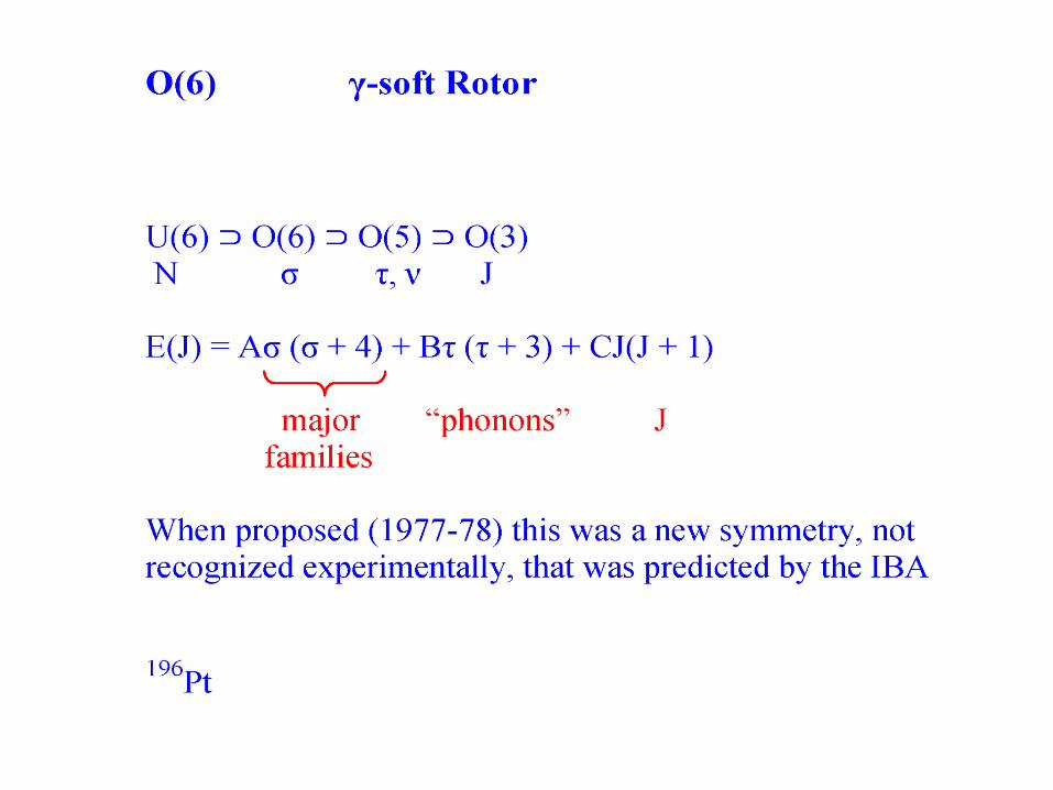
O(6) γ-soft

1

5U(6)

Sph.

Def.

Magical group

theory stuff

happens here

Symmetry Triangle of

the IBA

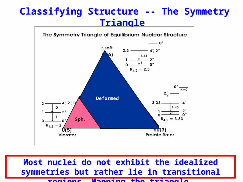
Classifying Structure -- The Symmetry Triangle

Most nuclei do not exhibit the idealized symmetries but rather lie in transitional regions. Mapping the triangle.

Sph.

Deformed

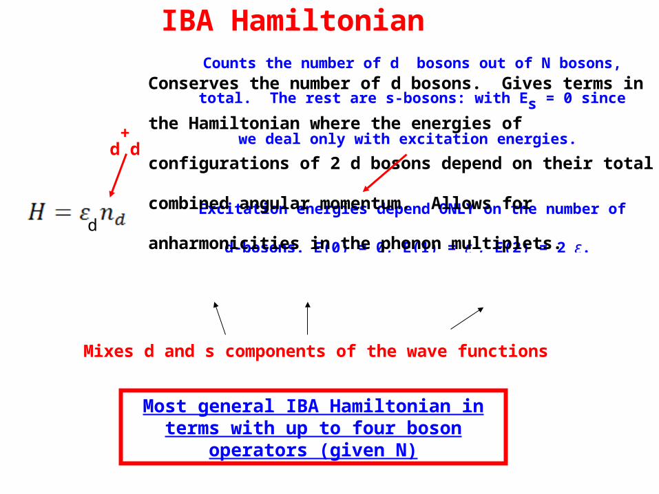
Most general IBA Hamiltonian in terms with up to four boson operators (given N)

IBA Hamiltonian

Mixes d and s components of the wave functions

d+

d

Counts the number of d bosons out of N bosons, total. The

rest are s-bosons: with Es = 0 since we deal only with

excitation energies.

Excitation energies depend ONLY on the number of d-bosons.

E(0) = 0, E(1) = ε , E(2) = 2 ε.

Conserves the number of d bosons. Gives terms in the

Hamiltonian where the energies of configurations of 2 d bosons

depend on their total combined angular momentum. Allows for

anharmonicities in the phonon multiplets.d

U(5)

Spherical, vibrational nuclei

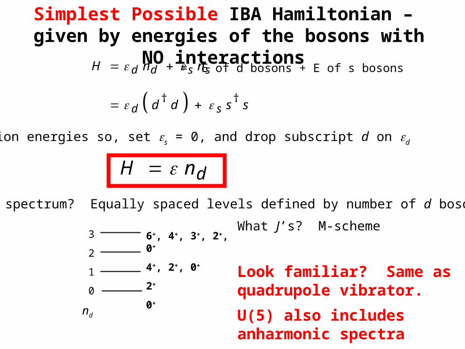
What J’s? M-scheme

Look familiar? Same as quadrupole vibrator.

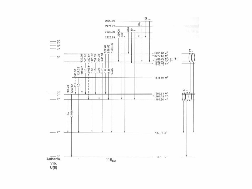
U(5) also includes anharmonic spectra

6+, 4+, 3+, 2+, 0+

4+, 2+, 0+

2+

0+

3

2

1

0

nd

Simplest Possible IBA Hamiltonian – given by energies of the bosons with NO interactions

† †

d d s s

d s

H n n

d d s s

Excitation energies so, set s = 0, and drop subscript d on d

dH n

What is spectrum? Equally spaced levels defined by number of d bosons

= E of d bosons + E of s bosons

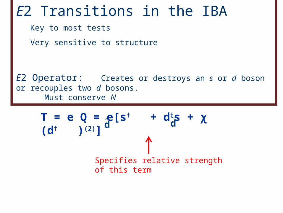
E2 Transitions in the IBAKey to most tests

Very sensitive to structure

E2 Operator: Creates or destroys an s or d boson or recouples two d bosons. Must conserve N

T = e Q = e[s† + d†s + χ (d† )(2)]d d

Specifies relative strength of this term

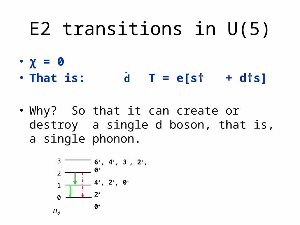
E2 transitions in U(5)

• χ = 0• That is: T = e[s† + d†s]

• Why? So that it can create or destroy a single d boson, that is, a single phonon.

d

6+, 4+, 3+, 2+, 0+

4+, 2+, 0+

2+

0+

3

2

1

0

nd

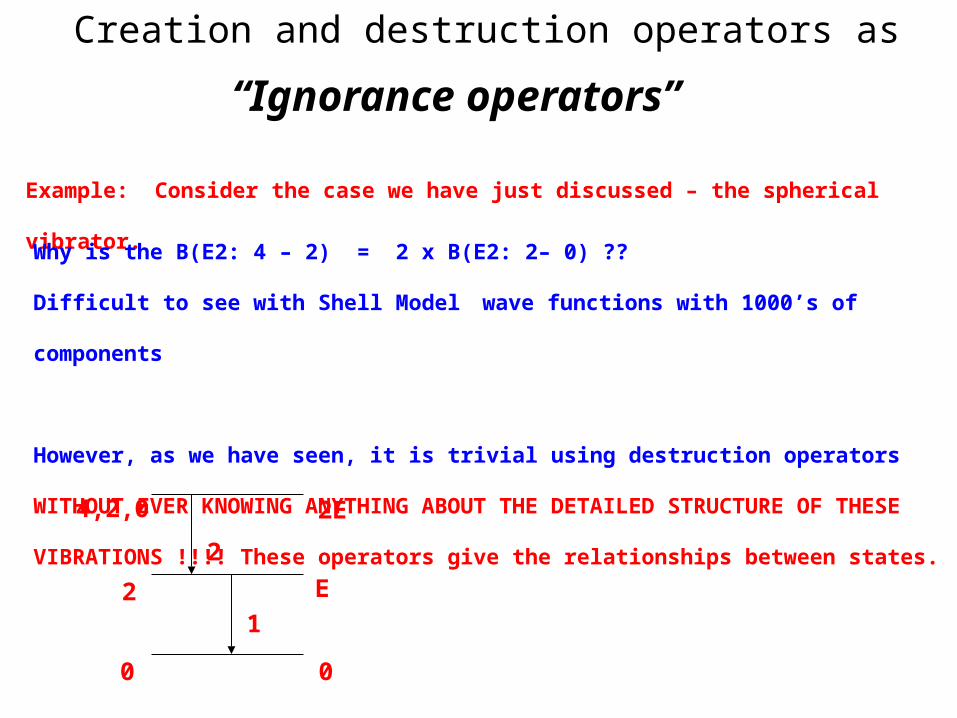
Creation and destruction operators as

Example: Consider the case we have just discussed – the spherical vibrator.

0

2

4,2,0

0

E

2E

1

2

Why is the B(E2: 4 – 2) = 2 x B(E2: 2– 0) ??

Difficult to see with Shell Model wave functions with 1000’s of components

However, as we have seen, it is trivial using destruction operators WITHOUT EVER

KNOWING ANYTHING ABOUT THE DETAILED STRUCTURE OF THESE VIBRATIONS !!!!

These operators give the relationships between states.

“Ignorance operators”

0+

2+

6+. . .

8+. . .

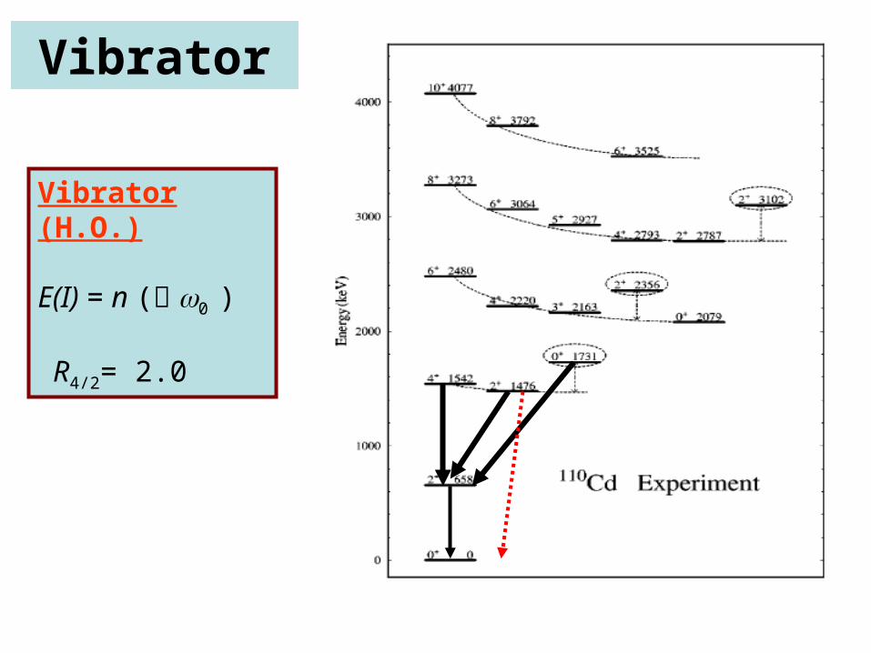
Vibrator (H.O.)

E(I) = n ( 0 )

R4/2= 2.0

Vibrator

Deformed nuclei

Use the same Hamiltonian but re-write it in more convenient and

physically intuitive form

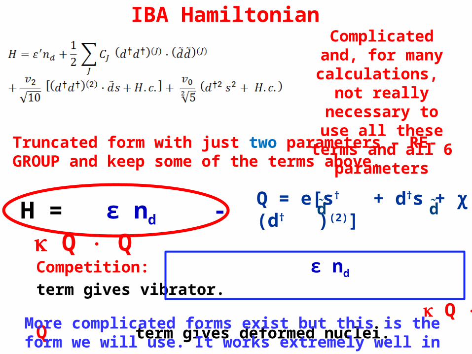
IBA HamiltonianComplicated and, for many calculations,

not really necessary to use all these terms

and all 6 parameters

Truncated form with just two parameters – RE-GROUP and keep some of the terms above.

H = ε nd - Q Q Q = e[s† + d†s + χ (d† )(2)]d d

Competition: ε nd term gives vibrator.

Q Q term gives deformed nuclei.

More complicated forms exist but this is the form we will use. It works extremely well in most cases.

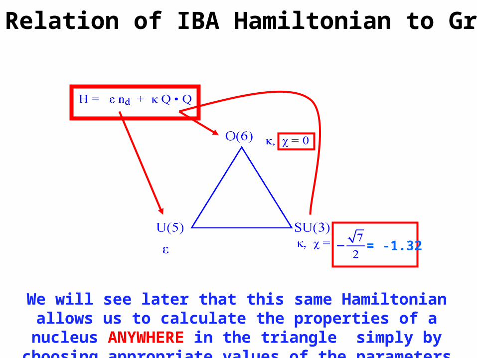
Relation of IBA Hamiltonian to Group Structure

We will see later that this same Hamiltonian allows us to calculate the properties of a nucleus ANYWHERE in the triangle simply by

choosing appropriate values of the parameters

= -1.32

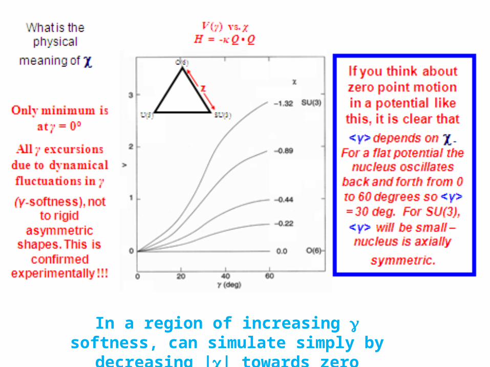
In a region of increasing g softness, can simulate simply by decreasing |c| towards zero

SU(3)

Deformed nuclei

Any calculation deviating from U(5) gives wave functions where nd is no longer a good quantum number. If the wave function is expressed in a

U(5) – vibrator – basis, then it contains a mixture of terms. Understanding these admixtures is crucial to understanding IBA

calculations

Effects of non-diagonal terms in HIBA

Recall So,

† † † † , 1s s sd dd d ds n n d d d n n n

† †

†

1, 1

, 1

1 1, 1

1 1, 1

sd d

sd d d

sd d d d

sd d d

s

s

s

s

d d n n n n

d n n n n n

n n n n n n

n n n n n

†

1

1 1b b b

b b b

b n n n

b n n n

2+

0+

2+ 4

+ 0+

† † mixingd d d s

Δ nd = 1 mixing

Wave functions in SU(3): Consider non-diagonal effects of the QQ term in H on nd components in the wave functions

Q operator: Q = (s† d + d †s) + (d † d )(2)

QQ = [ { (s† d + d †s) + χ(d †d ) (2) } x { (s† d + d †s) + (d †d )(2) } ]

~ s† d s† d + s† d d †s + s† d d † d …. D nd = -2 0 -1 …. 2, 0, 1

72

72

M

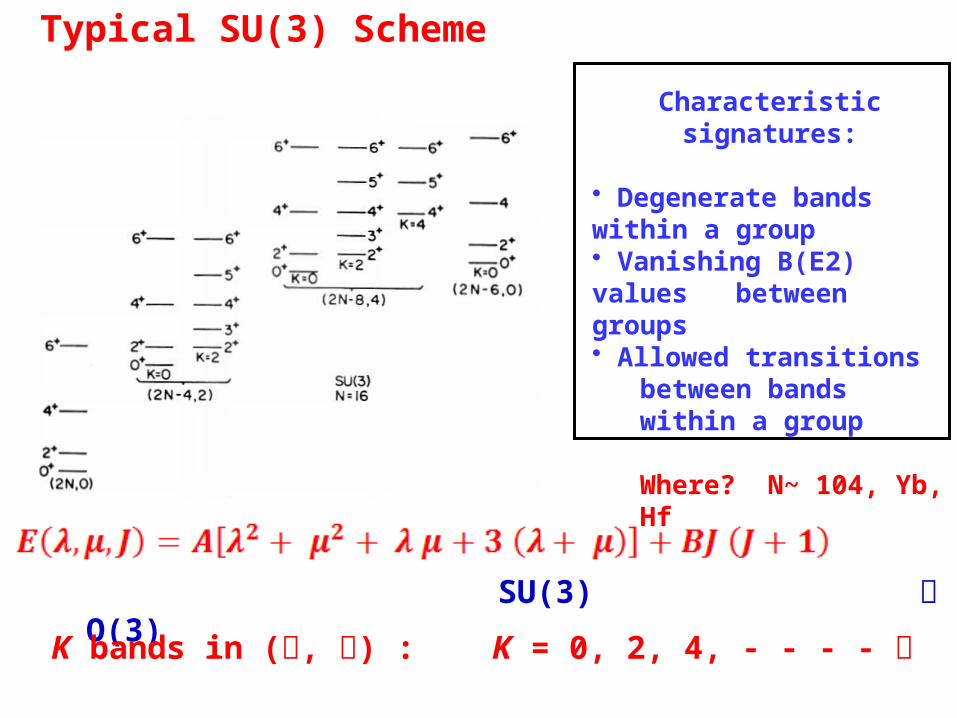
Typical SU(3) Scheme

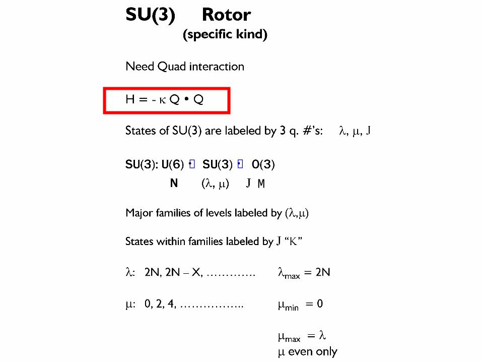
SU(3) O(3)

K bands in (, ) : K = 0, 2, 4, - - - -

Characteristic signatures:

• Degenerate bands within a group• Vanishing B(E2) values

between groups• Allowed transitions

between bands within a group

Where? N~ 104, Yb, Hf

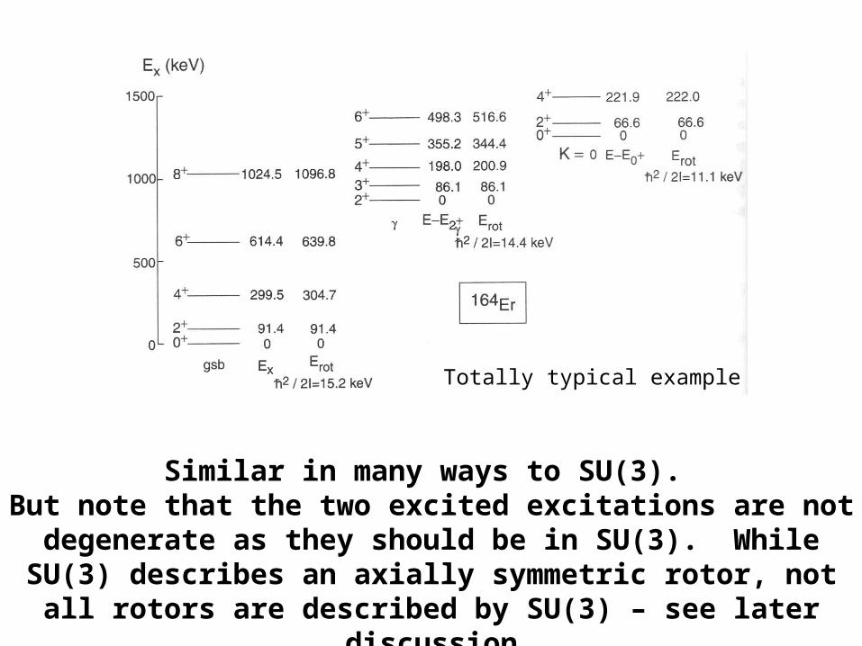
Totally typical example

Similar in many ways to SU(3). But note that the two excited excitations are not degenerate as they should be in SU(3). While SU(3) describes an axially symmetric rotor,

not all rotors are described by SU(3) – see later discussion

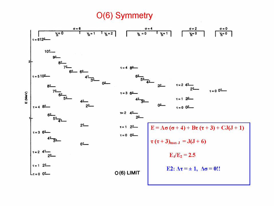
O(6)

Axially asymmetric nuclei(gamma-soft)

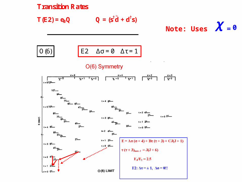
Transition Rates

T(E2) = eBQ Q = (s†d + d†s)

B(E2; J + 2 → J) = 2B

J+ 1

24

J Je N - N2 2 J + 5

B(E2; 21 → 01) ~ 2B

+ 4e

5N N

N2

Consider E2 selection rules Δσ = 0 0+(σ = N - 2) – No allowed decays! Δτ = 1 0+( σ = N, τ = 3) – decays to 22 , not 12

O(6) E2 Δσ = 0 Δτ = 1

Note: Uses χ = 0

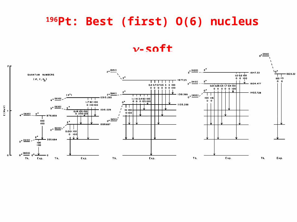
196Pt: Best (first) O(6) nucleus -soft

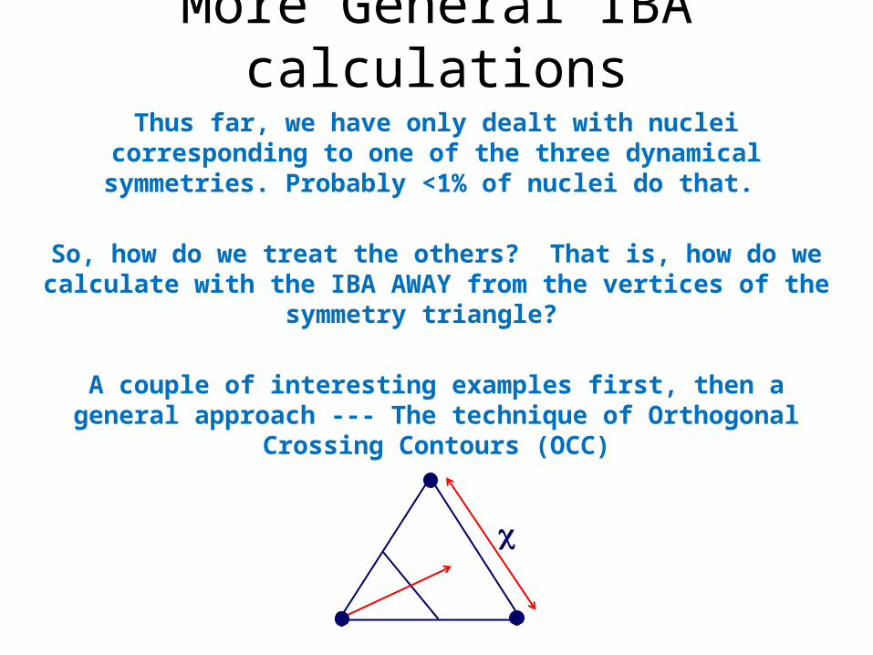
Thus far, we have only dealt with nuclei corresponding to one of the three dynamical symmetries. Probably <1% of nuclei do that.

So, how do we treat the others? That is, how do we calculate with the IBA AWAY from the vertices of the symmetry triangle?

A couple of interesting examples first, then a general approach --- The technique of Orthogonal Crossing Contours (OCC)

More General IBA calculations

c

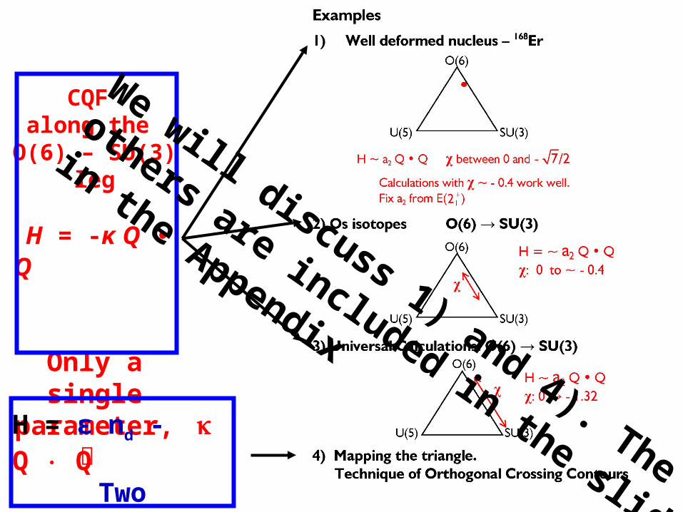
CQF along the

O(6) – SU(3) leg

H = -κ Q • Q

Only a single parameter,

H = ε nd - Q Q Two parameters

ε / and

We will discuss 1) and 4). The others are

included in the slides in the Appendix

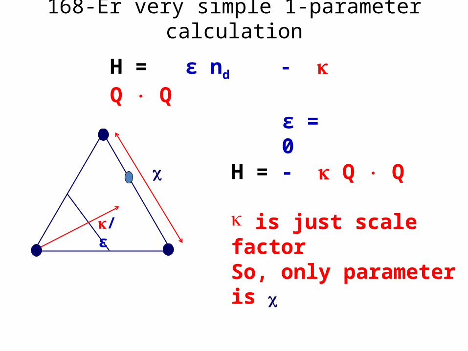
c

H = ε nd - Q Q

ε = 0

/ε

168-Er very simple 1-parameter calculation

H = - Q Q

k is just scale factorSo, only parameter is c

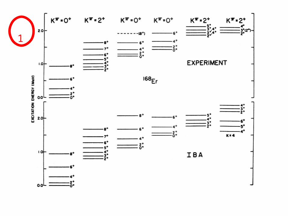
1

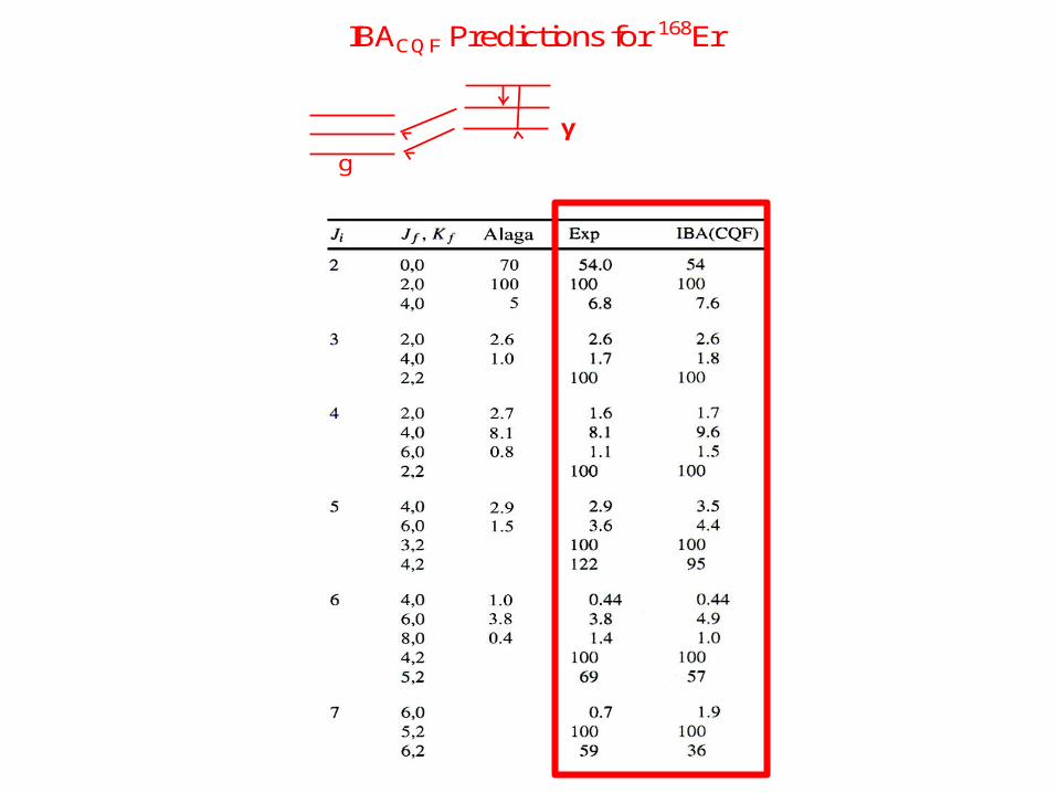
IBACQF Predictions for 168Er

γ

g

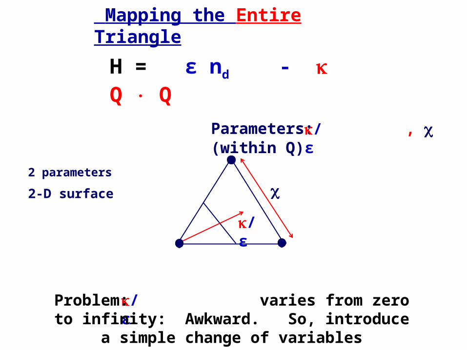
Mapping the Entire Triangle

2 parameters

2-D surface c

H = ε nd - Q Q

Parameters: , c (within Q) /ε

/ε

/ε Problem: varies from zero to infinity: Awkward. So, introduce a simple change of variables

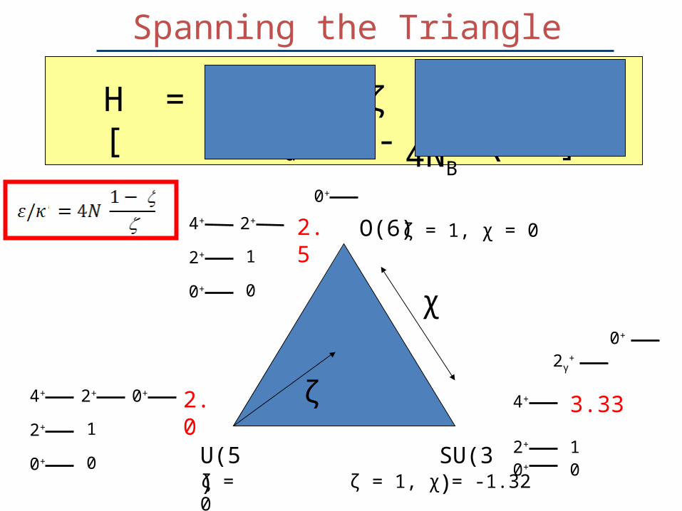
Spanning the Triangle

H = c [

ζ ( 1 – ζ ) nd

4NB

Qχ ·Qχ - ]

ζ

χ

U(5)0+

2+ 0+

2+

4+

0

2.01

ζ = 0

O(6)

0+

2+

0+

2+

4+

0

2.51

ζ = 1, χ = 0

SU(3)

2γ+

0+

2+

4+ 3.33

10+ 0

ζ = 1, χ = -1.32

2 3 5

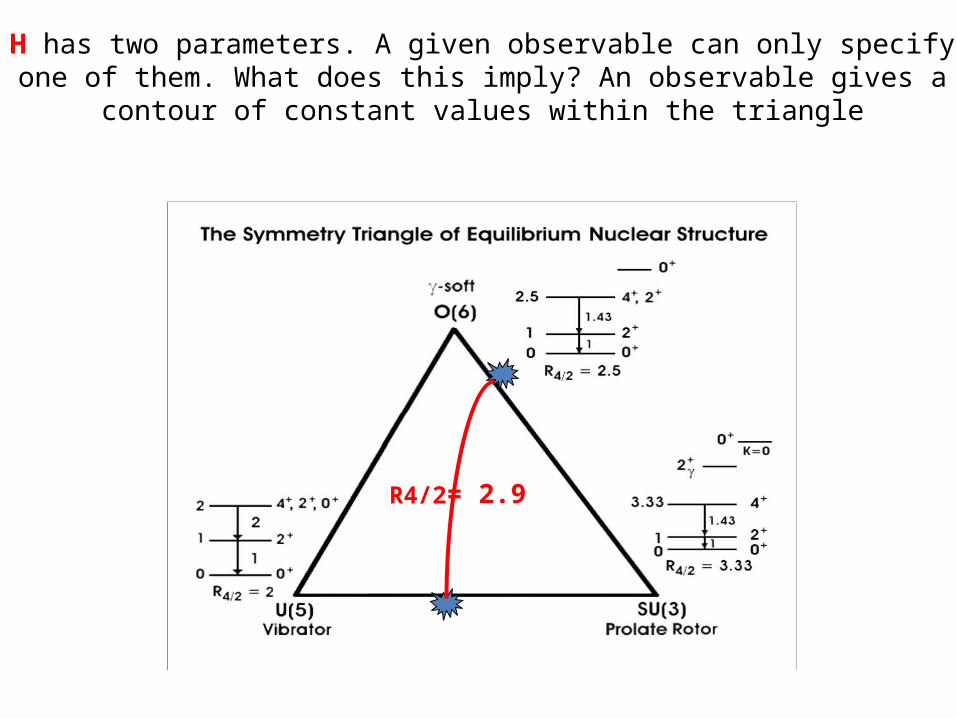
H has two parameters. A given observable can only specify one of them. What does this imply? An observable gives a contour of constant values

within the triangle

= 2.9R4/2

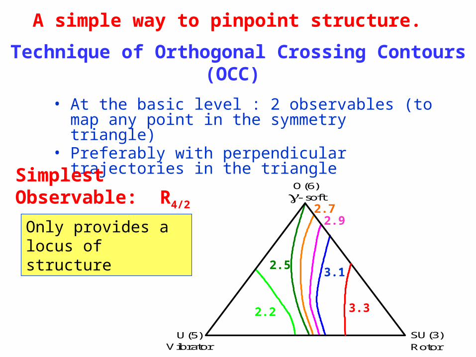
• At the basic level : 2 observables (to map any point in the symmetry triangle)

• Preferably with perpendicular trajectories in the triangle

A simple way to pinpoint structure.

Technique of Orthogonal Crossing Contours (OCC)

Simplest Observable: R4/2

Only provides a locus of structure

Vibrator Rotor

- soft

U(5) SU(3)

O(6)

3.3

3.1

2.92.7

2.5

2.2

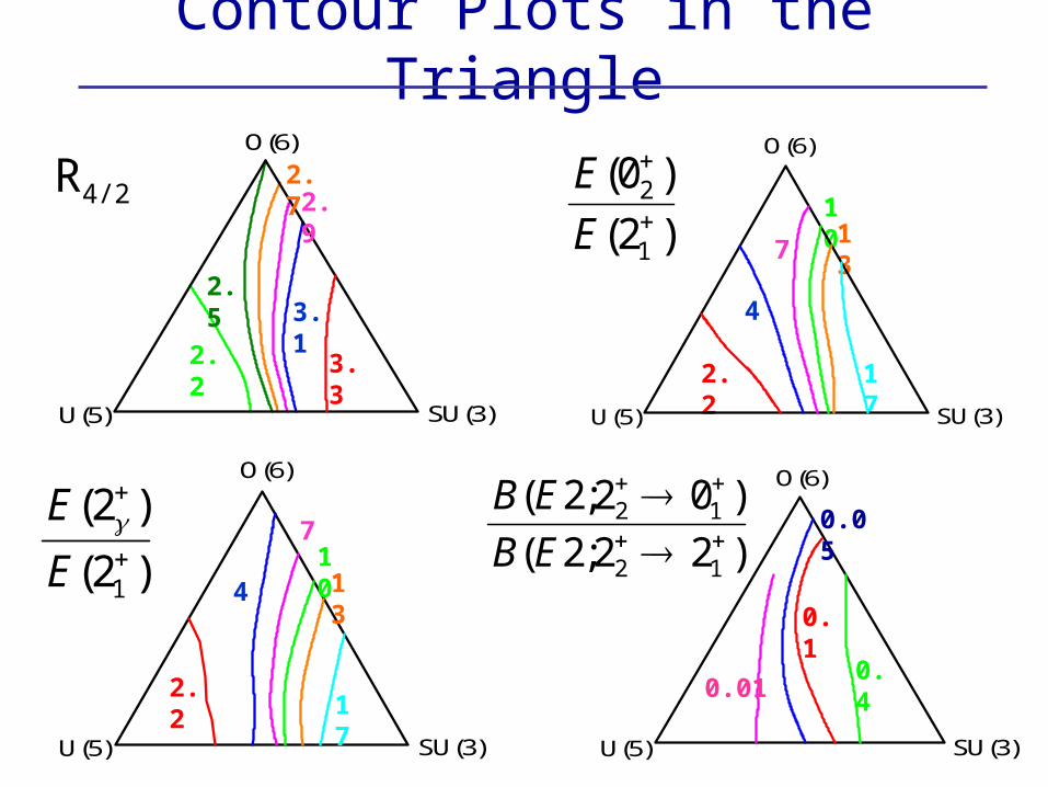
Contour Plots in the Triangle

U(5) SU(3)

O(6)

3.3

3.1

2.92.7

2.5

2.2

R4/2

SU(3)U(5)

O(6)

2.2

4

7

1310

17

2.2

4

7

1013

17

SU(3)U(5)

O(6)

SU(3)U(5)

O(6)

0.1

0.05

0.010.4

)2(

)2(

1

E

E

)2(

)0(

1

2

E

E

)22;2(

)02;2(

12

12

EB

EB

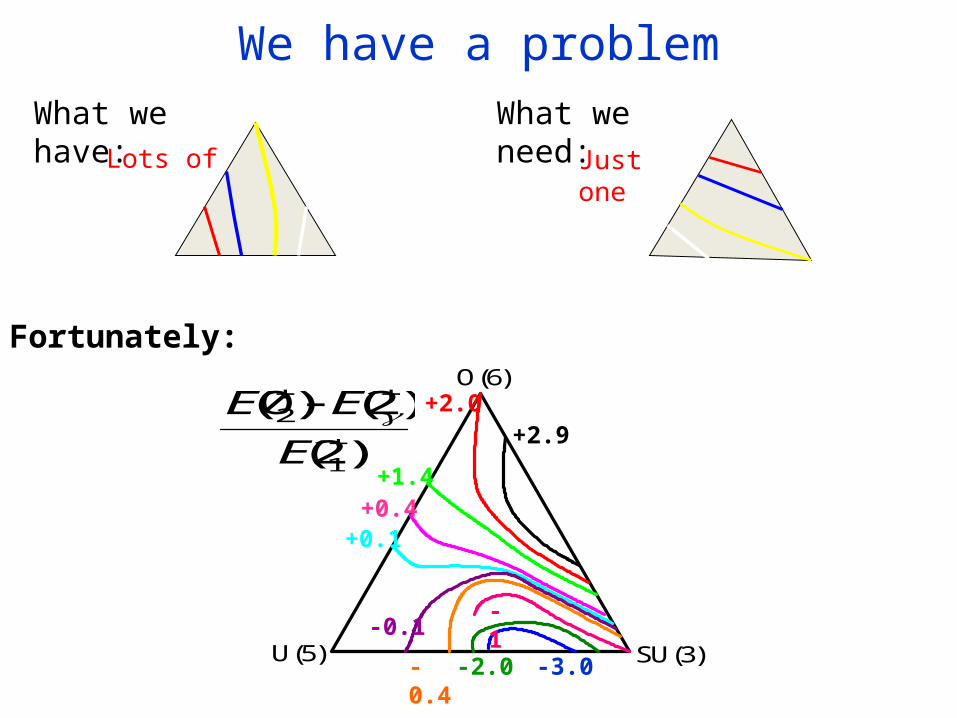
We have a problemWhat we have:

Lots of

What we need:

Just one

U(5) SU(3)

O(6)

+2.9+2.0

+1.4+0.4

+0.1

-0.1

-0.4

-1

-2.0 -3.0

)2(

)2()0(

1

2

E

EE

Fortunately:

)2(

)2()0(

1

22

E

EE)2(

)4(

1

1

E

EVibrator Rotor

γ - soft

Mapping Structure with Simple Observables – Technique of Orthogonal Crossing Contours

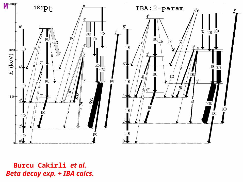
Burcu Cakirli et al.Beta decay exp. + IBA calcs.

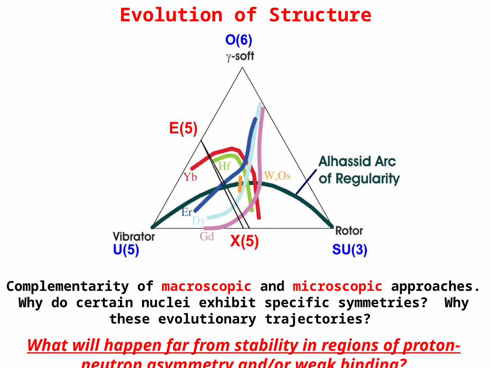
Evolution of Structure

Complementarity of macroscopic and microscopic approaches. Why do certain nuclei exhibit specific symmetries? Why these evolutionary trajectories?

What will happen far from stability in regions of proton-neutron asymmetry and/or weak binding?

Special Thanks to:

• Franco Iachello• Akito Arima• Igal Talmi• Dave Warner• Peter von Brentano• Victor Zamfir• Jolie Cizewski• Hans Borner• Jan Jolie• Burcu Cakirli• Piet Van Isacker• Kris Heyde • Many others

Appendix:

Trajectories-by-eye

Running the IBA program using the Titan computer at Yale

Examples “2” and “3” skipped earlier of the use of the CQF form

of the IBA

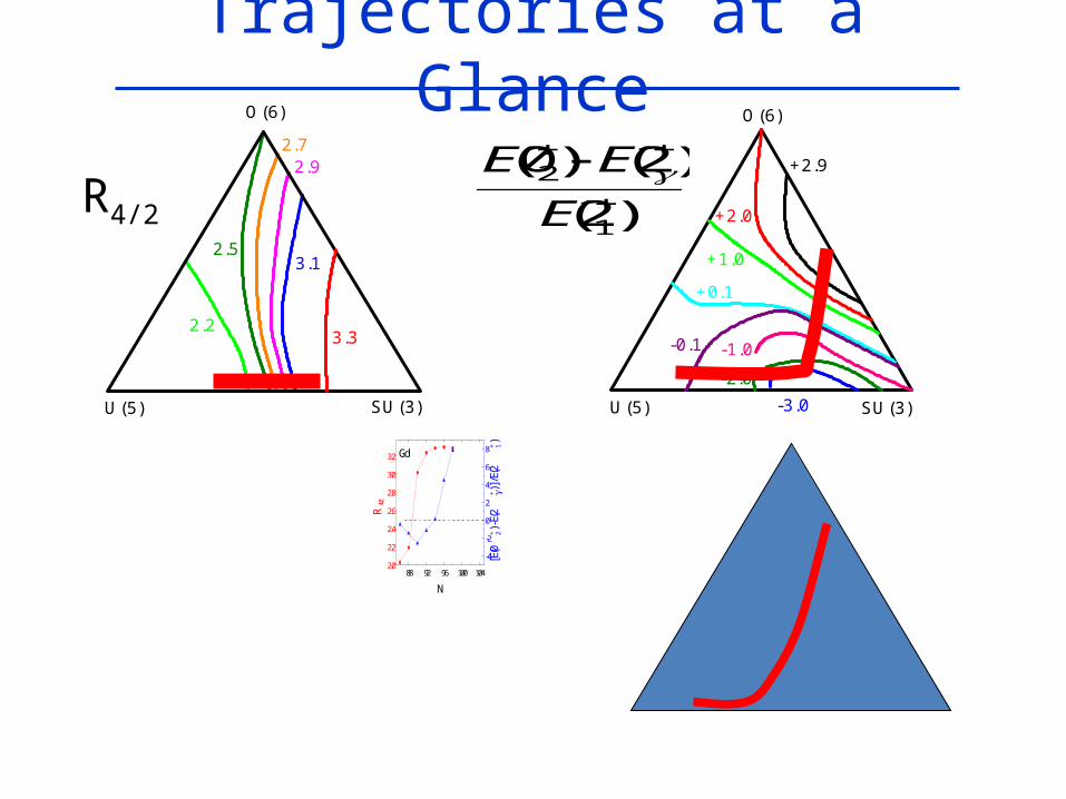
Trajectories at a Glance

88 92 96 100 1042.0

2.2

2.4

2.6

2.8

3.0

3.2 Gd

N

R4/2

-4

-2

0

2

4

6

8

[ E(0

+ 2) - E

(2+ )

] / E(2

+ 1)

-3.0

-1.0-2.0

-0.1

+0.1

+1.0

+2.0

+2.9

U(5) SU(3)

O(6)

SU(3)U(5)

O(6)

3.3

3.1

2.92.7

2.5

2.2

R4/2 )2(

)2()0(

1

2

E

EE

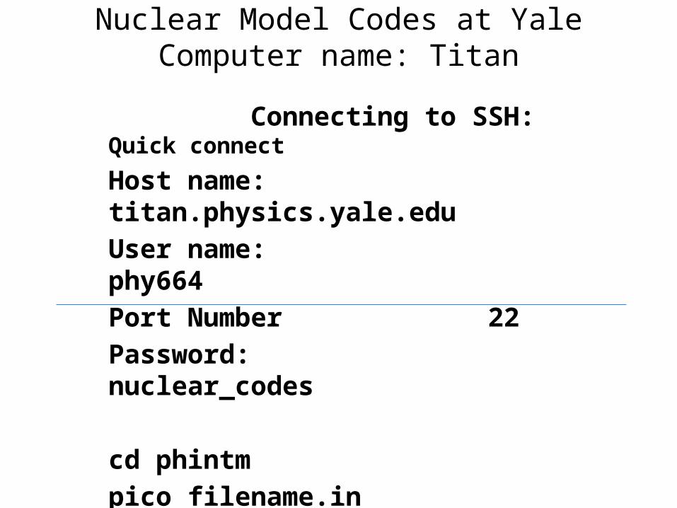
Nuclear Model Codes at YaleComputer name: Titan

Connecting to SSH: Quick connect

Host name: titan.physics.yale.eduUser name: phy664Port Number 22Password: nuclear_codes

cd phintmpico filename.in (ctrl x, yes, return)runphintm filename (w/o extension)pico filename.out (ctrl x, return)

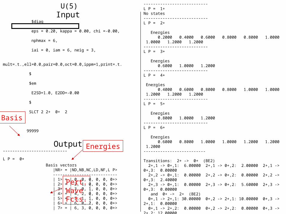
Input $diag eps = 0.20, kappa = 0.00, chi =-0.00, nphmax = 6, iai = 0, iam = 6, neig = 3, mult=.t.,ell=0.0,pair=0.0,oct=0.0,ippm=1,print=.t. $ $em E2SD=1.0, E2DD=-0.00 $ SLCT 2 2+ 0+ 2 99999

Output---------------------------

L P = 0+

Basis vectors |NR> = |ND,NB,NC,LD,NF,L P> --------------------------- | 1> = | 0, 0, 0, 0, 0, 0+> | 2> = | 2, 1, 0, 0, 0, 0+> | 3> = | 3, 0, 1, 0, 0, 0+> | 4> = | 4, 2, 0, 0, 0, 0+> | 5> = | 5, 1, 1, 0, 0, 0+> | 6> = | 6, 0, 2, 0, 0, 0+> | 7> = | 6, 3, 0, 0, 0, 0+>

Energies 0.0000 0.4000 0.6000 0.8000 1.0000 1.2000 1.2000

Eigenvectors

1: 1.000 0.000 0.000 2: 0.000 1.000 0.000 3: 0.000 0.000 1.000 4: 0.000 0.000 0.000 5: 0.000 0.000 0.000 6: 0.000 0.000 0.000 7: 0.000 0.000 0.000

---------------------------L P = 1+No states---------------------------L P = 2+

Energies 0.2000 0.4000 0.6000 0.8000 0.8000 1.0000 1.0000 1.2000 1.2000---------------------------L P = 3+ Energies 0.6000 1.0000 1.2000---------------------------L P = 4+

Energies 0.4000 0.6000 0.8000 0.8000 1.0000 1.0000 1.2000 1.2000 1.2000---------------------------L P = 5+ Energies 0.8000 1.0000 1.2000 ---------------------------L P = 6+ Energies 0.6000 0.8000 1.0000 1.0000 1.2000 1.2000 1.2000--------------------------

Transitions: 2+ -> 0+ (BE2) 2+,1 -> 0+,1: 6.00000 2+,1 -> 0+,2: 2.00000 2+,1 -> 0+,3: 0.00000 2+,2 -> 0+,1: 0.00000 2+,2 -> 0+,2: 0.00000 2+,2 -> 0+,3: 2.40000 2+,3 -> 0+,1: 0.00000 2+,3 -> 0+,2: 5.60000 2+,3 -> 0+,3: 0.00000 and 0+ -> 2+ (BE2) 0+,1 -> 2+,1: 30.00000 0+,2 -> 2+,1: 10.00000 0+,3 -> 2+,1: 0.00000 0+,1 -> 2+,2: 0.00000 0+,2 -> 2+,2: 0.00000 0+,3 -> 2+,2: 12.00000 0+,1 -> 2+,3: 0.00000 0+,2 -> 2+,3: 28.00000 0+,3 -> 2+,3: 0.00000

Transitions: 4+ -> 2+ (BE2) 4+,1 -> 2+,1: 10.00000 4+,1 -> 2+,2: 0.00000 4+,1 -> 2+,3: 2.28571 4+,2 -> 2+,1: 0.00000 4+,2 -> 2+,2: 6.28571 4+,2 -> 2+,3: 0.00000 4+,3 -> 2+,1: 0.00000 4+,3 -> 2+,2: 0.00000 4+,3 -> 2+,3: 3.85714

U(5)

Basis

Energies

Pert.WaveFcts.

Input

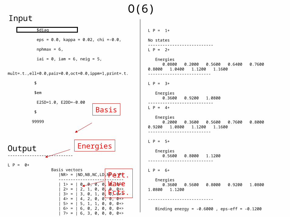
$diag eps = 0.0, kappa = 0.02, chi =-0.0, nphmax = 6, iai = 0, iam = 6, neig = 5, mult=.t.,ell=0.0,pair=0.0,oct=0.0,ippm=1,print=.t. $ $em E2SD=1.0, E2DD=-0.00 $ 99999

Output---------------------------

L P = 0+ Basis vectors |NR> = |ND,NB,NC,LD,NF,L P> --------------------------- | 1> = | 0, 0, 0, 0, 0, 0+> | 2> = | 2, 1, 0, 0, 0, 0+> | 3> = | 3, 0, 1, 0, 0, 0+> | 4> = | 4, 2, 0, 0, 0, 0+> | 5> = | 5, 1, 1, 0, 0, 0+> | 6> = | 6, 0, 2, 0, 0, 0+> | 7> = | 6, 3, 0, 0, 0, 0+>

Energies 0.0000 0.3600 0.5600 0.9200 0.9600 1.0800 1.2000

Eigenvectors

1: -0.433 0.000 0.685 0.000 0.559 2: -0.750 0.000 0.079 0.000 -0.581 3: 0.000 -0.886 0.000 0.463 0.000 4: -0.491 0.000 -0.673 0.000 0.296 5: 0.000 -0.463 0.000 -0.886 0.000 6: 0.000 0.000 0.000 0.000 0.000 7: -0.094 0.000 -0.269 0.000 0.512---------------------------

L P = 1+

No states---------------------------L P = 2+ Energies 0.0800 0.2000 0.5600 0.6400 0.7600 0.8000 1.0400 1.1200 1.1600--------------------------

L P = 3+ Energies 0.3600 0.9200 1.0800---------------------------L P = 4+ Energies 0.2000 0.3600 0.5600 0.7600 0.8000 0.9200 1.0800 1.1200 1.1600--------------------------

L P = 5+

Energies 0.5600 0.8000 1.1200---------------------------

L P = 6+ Energies 0.3600 0.5600 0.8000 0.9200 1.0800 1.0800 1.1200

---------------------------

Binding energy = -0.6000 , eps-eff = -0.1200

O(6)

Basis

Pert.WaveFcts.

Energies

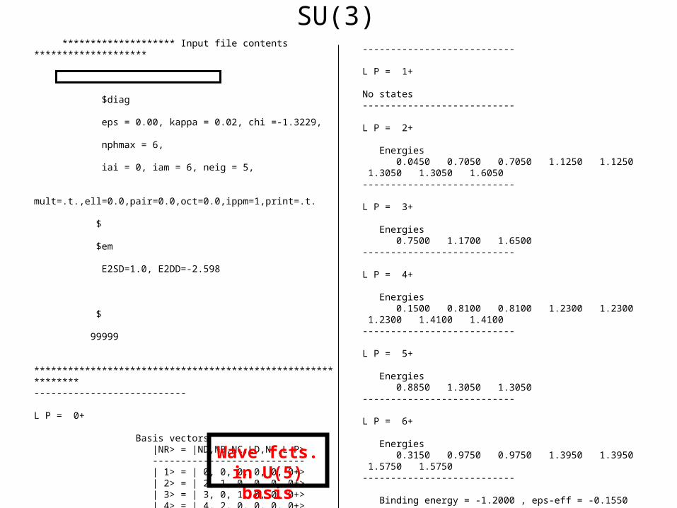
******************** Input file contents ******************** $diag eps = 0.00, kappa = 0.02, chi =-1.3229, nphmax = 6, iai = 0, iam = 6, neig = 5, mult=.t.,ell=0.0,pair=0.0,oct=0.0,ippm=1,print=.t. $ $em E2SD=1.0, E2DD=-2.598 $ 99999 *************************************************************---------------------------

L P = 0+

Basis vectors |NR> = |ND,NB,NC,LD,NF,L P> --------------------------- | 1> = | 0, 0, 0, 0, 0, 0+> | 2> = | 2, 1, 0, 0, 0, 0+> | 3> = | 3, 0, 1, 0, 0, 0+> | 4> = | 4, 2, 0, 0, 0, 0+> | 5> = | 5, 1, 1, 0, 0, 0+> | 6> = | 6, 0, 2, 0, 0, 0+> | 7> = | 6, 3, 0, 0, 0, 0+>

Energies 0.0000 0.6600 1.0800 1.2600 1.2600 1.5600 1.8000

Eigenvectors

1: 0.134 0.385 -0.524 -0.235 0.398 2: 0.463 0.600 -0.181 0.041 -0.069 3: -0.404 -0.204 -0.554 -0.557 -0.308 4: 0.606 -0.175 0.030 -0.375 -0.616 5: -0.422 0.456 -0.114 0.255 -0.432 6: -0.078 0.146 -0.068 0.245 -0.415 7: 0.233 -0.437 -0.606 0.606 0.057

---------------------------

L P = 1+

No states---------------------------

L P = 2+

Energies 0.0450 0.7050 0.7050 1.1250 1.1250 1.3050 1.3050 1.6050 ---------------------------

L P = 3+ Energies 0.7500 1.1700 1.6500---------------------------

L P = 4+ Energies 0.1500 0.8100 0.8100 1.2300 1.2300 1.2300 1.4100 1.4100 ---------------------------

L P = 5+ Energies 0.8850 1.3050 1.3050---------------------------

L P = 6+

Energies 0.3150 0.9750 0.9750 1.3950 1.3950 1.5750 1.5750---------------------------

Binding energy = -1.2000 , eps-eff = -0.1550

SU(3)

Wave fcts. in U(5) basis

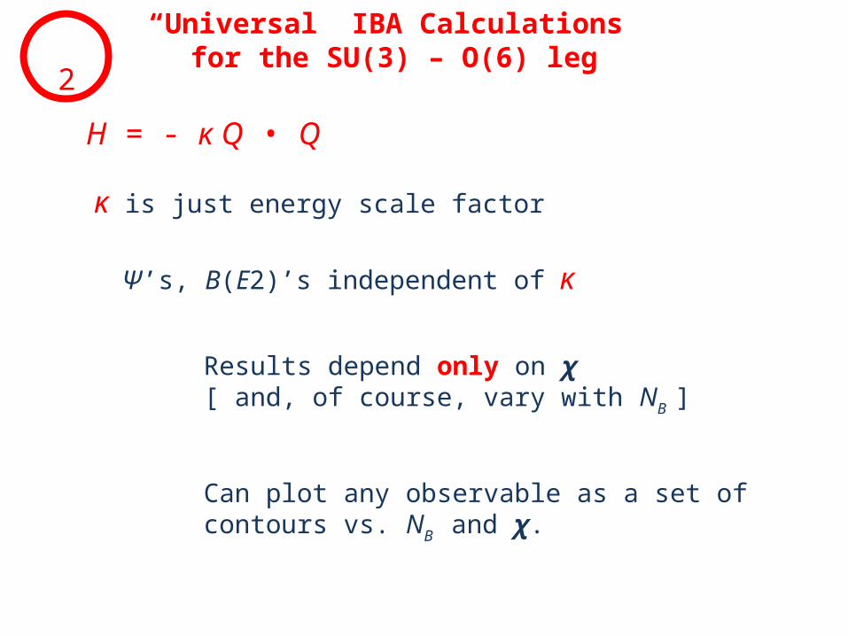
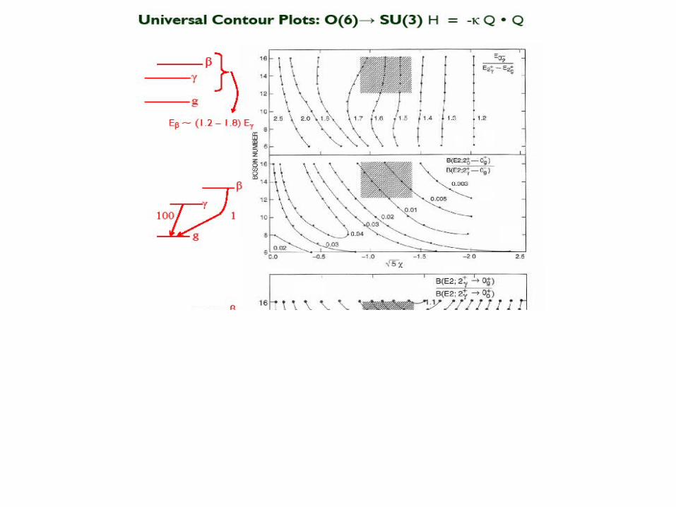
“Universal” IBA Calculations for the SU(3) – O(6) leg

H = - κ Q • Q

κ is just energy scale factor

Ψ’s, B(E2)’s independent of κ

Results depend only on χ [ and, of course, vary with NB ]

Can plot any observable as a set of contours vs. NB and χ.

2

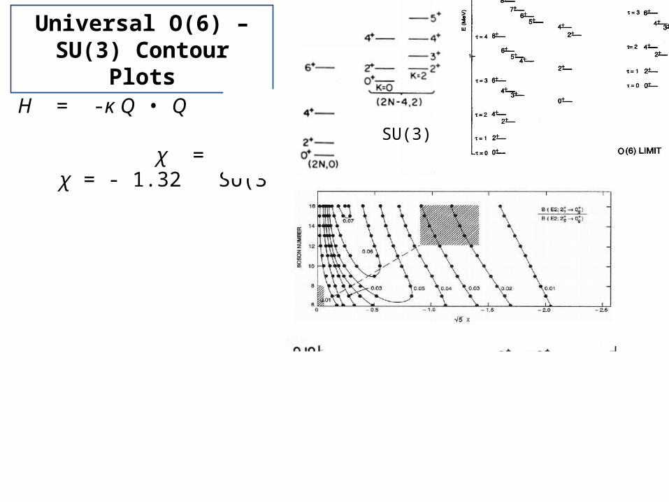
Universal O(6) – SU(3) Contour Plots

H = -κ Q • Q

χ = 0 O(6) χ = - 1.32 SU(3)

SU(3)

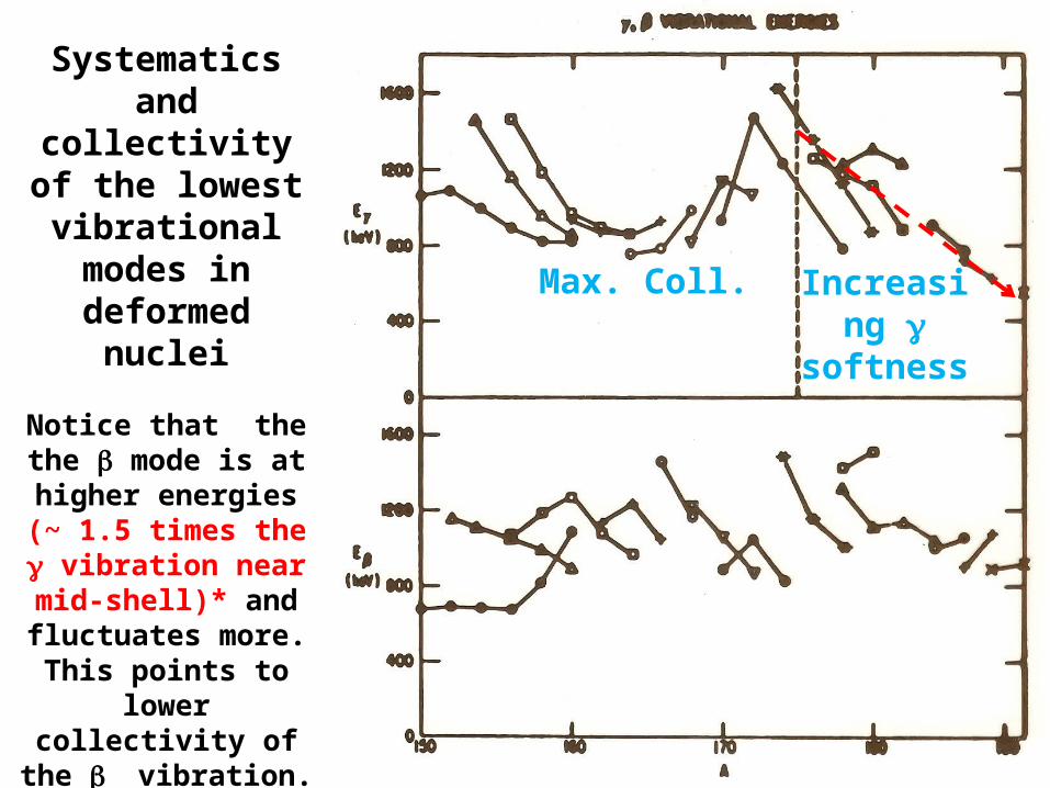
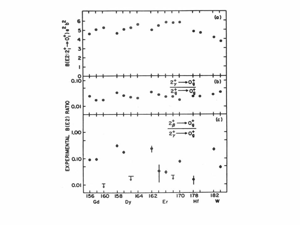
Systematics and collectivity of the lowest vibrational

modes in deformed nuclei

Notice that the the b mode is at higher

energies (~ 1.5 times the g vibration near

mid-shell)* and fluctuates more. This

points to lower collectivity of the b

vibration.

* Remember for later !

Max. Coll. Increasing g softness

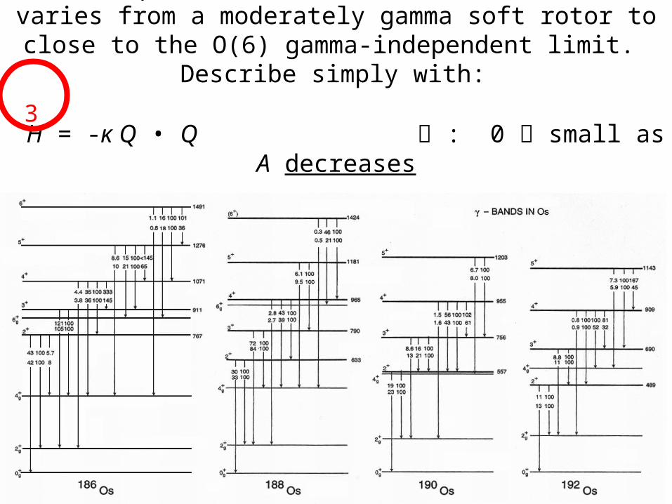
Os isotopes from A = 186 to 192: Structure varies from a moderately gamma soft rotor to close to the O(6) gamma-

independent limit. Describe simply with:

H = -κ Q • Q : 0 small as A decreases3

End of Appendix