Embed Size (px)
Citation preview

SPIS TREŚCI
1EKSPLOATACJA I NIEZAWODNOŚĆ NR 2/2006
Nauka i Technika
Y. Vidya KIRAN, Biswajit MAHANTYReliability Design of Embedded Systems .....................................................................................4
Kailash C. KAPURMulti-state Reliability: Models and Applications ..........................................................................8
Milan HOLICKÝFuzzy probabilistic models in structural reliability .......................................................................11
Rose D. BAKERRisk Aversion in Maintenance ...................................................................................................14
Igor A. USHAKOVTerrestrial Maintenance System for Geographically Distributed Clients ........................................17
Anatoly LISNIANSKI, David LAREDO, Hanoch Ben HAIMRedundant Systems Shutdown During Low Capacity Operation ...................................................23
Radim BRIŠ, Pavel PRAAKSSimulation Approach for Modeling of Dynamic Reliability using Time Dependent Acyclic Graph......26
Elena ZAITSEVA, Vitaly LEVASHENKO, Karol MATIAŠKOFailure Analysis of Series and Parallel Multi-State System ..........................................................29
Enrico ZIO, Luca PODOFILLINIThe Use of Importance Measures for the Optimization of Multi-State Systems ..............................33
Ilia FRENKEL, Lev KHVATSKINCost – effective maintenance with preventive replacement of oldest components .........................37
Alexander ROTSHTEIN, Serhiy SHTOVBAModeling of Algorithmic Process Reliability with Fuzzy Source Data .............................................40
Boyan DIMITROV, David GREEN, Vladimir RYKOV, Peter STANCHEVOn the Fair Share of the Reliability of an Entity between its Components........................................ 44
Léo GERVILLE-RÉACHE, Mikhail NIKULINOn Statistical Modelling in Accelerated Life Testing .......................................................................48
Andrzej NIEWCZAS, Grzegorz KOSZAŁKA, Pawel DROŹDZIELStochastic model of truck engine wear with regard to discontinuity of operation.............................52

W SKRÓCIE
2 EKSPLOATACJA I NIEZAWODNOŚĆ NR 2/2006
KIRAN Y.V., MAHANTY B.: Reliability Design of Embedded Systems; EiN nr 2/2006, s. 4-7.
In the current era, the role of smart devices is expanding every day. These devices depend on both software and hardware functions to produce the desired results. The success of such devices depends on a new design paradigm that considers reliability in virtually every aspect of the devices’ software and hardware content. Design of a hardware system involves selection from numerous discrete choices among available component types based on cost, reliability, performance, weight, etc. Design of software systems involves the selection of the best choice from a stack of available choices with variable reliabilities and costs. We try to design an embedded system which optimizes the reliability in the perspective of cost or vice versa. An Integer Programming approach for simplifi ed assumptions and an Evolutionary approach for the non-simplifi ed case is proposed.
KAPUR K. C.: Multi-state Reliability: Models and Applications; EiN nr 2/2006, s. 8-10.
This paper focuses on customer-centered reliability models and measures for multi-state systems with multi-state components. A review of general models which capture the customer’s experience with the product is presented. An approach is given to develop the system structure function using equivalent classes and develop reliability bonds. In addition to measures and models, ideas are given for potential applications of these models to infrastructure problems such as transportation, computer network, supply chain, communication systems and network reliability.
HOLICKÝ M.: Fuzzy probabilistic models in structural reliability; EiN nr 2/2006, s. 11-13.
Two types of uncertainties can be generally recognised in structural reliability: natural randomness of basic variables and vagueness of performance requirements. While the randomness of basic variables is handled by common methods of the probability theory, the vagueness of the performance requirements is described by the basic tools of the theory of fuzzy sets. Both the types of uncertainties are combined in the newly defi ned fuzzy probabilistic measures of structural reliability, the damage function and the fuzzy probability of failure. The proposed measures can be effi ciently applied in a similar way as conventional probabilistic quantities for the verifi cation and optimisation of structural reliability. Adequate data are however needed for further development of the outlined concepts.
BAKER R., D.: Risk Aversion in Maintenance; EiN nr 2/2006, s. 14-16.
The concept of risk averse maintenance is introduced. It is formulated in terms of seeking to minimize a disutility rather than a cost per unit time. A general formalism is given, fol-lowed by an example, the application to age-based replacement. The problem of overmaintenance caused by undue risk aversion on the part of engineers is briefl y discussed.
USHAKOV I., A.: Terrestrial Maintenance System for Geographically Distributed Clients; EiN nr 2/2006, s. 17-22.
Clients (for instance, owners of ground equipment for satellite telecommunication network) are arbitrarily distributed on some territory. For maintenance/repair service, one uses Mobile Maintenance Stations (MMS) located at some Maintenance Bases (MB). The problem is to construct such maintenance zones which need minimum total number of MMS under condition that the Quality of Service (QoS) is not worse than required. A heuristic mathematical model of optimal zoning is suggested. An illustrative numerical example of constructing service zone for Florida State (USA) is given.
LISNIANSKI A., LAREDO D., HAIM H., B.: Redundant Systems Shutdown During Low Capacity Operation; EiN nr 2/2006, s. 23-25.
Two possible operation modes of various pumps with redundancy in electric power generating units during low load periods (night) were analyzed. The fi rst mode – two of three pumps work at night with 25% of nominal capacity, the third pump is a cold (passive) reserve. The second mode – one pump works at night with 50% of nominal capacity, two pumps are in cold reserve. A Markov reward model was built for the comparison analysis of these possible operation modes. The model takes into account all important factors – pumps power consumption, pumps failure rate, pumps starting availability, cost of alternative energy, and penalty cost of energy not supplied. It was shown that under current operation conditions the second operation mode is more effective one.
BRIŠ R., PRAAKS P.: Simulation Approach for Modeling of Dynamic Reliability using Time Dependent Acyclic Graph; EiN nr 2/2006, s. 26-28.
The dynamic reliability approach takes into account changes (evolution) of the system structure (hardware). For instance, the dynamic reliability allows modeling a human ope-rator (or an electronic control system) naturally. In these cases, the structure of the system is usually changed in order to keep the functionality and/or safety of the system. The main purpose of the paper is to illustrate, by means of a model example, the ability of acyclic oriented graph, terminal nodes of which are programmable components, to model simple dynamic system and to assess its performance via Monte-Carlo simulations. To demonstrate the availability of our framework a test case study with the deterministic evolution is presented. The here presented numerical results are in agreement with the exact analytical solution.
ZAITSEVA E., LEVASHENKO V., MATIAŠKO K.: Failure Analysis of Series and Parallel Multi-State System; EiN nr 2/2006, s. 29-32.
The reliability of the Multi-State System is investigated by Dynamic Reliability Indices in this paper. These indices estimate infl uence upon the Multi-State System reliability by the state of a system component. Structure function and mathematical tools of Multiple-Valued Logic calculate them. Dynamic Reliability Indices for failure of parallel and series systems are examined in detail.
ZIO E., PODOFILLINI L.: The Use of Importance Measures for the Optimization of Multi-State Systems; EiN nr 2/2006, s. 33-36.
In this paper we propose an approach to the multiobjective optimization of a multi-state system (MSS) design, based on incorporating information from importance measures (IMs). More specifi cally, IMs come into play at the objective functions level in order to drive the search towards a MSS which, besides being optimal from the points of view of economics and safety, is also ‘balanced’ in the sense that all components have similar IMs values, without bottlenecks or unnecessarily high-performing components.
FRENKEL I., KHVATSKIN L.: Cost – effective maintenance with preventive replacement of oldest components; EiN nr 2/2006, s. 37-39.
We consider preventive maintenance of a continuously operating system, whose real-life prototype is a rotating chemical reactor for production of phosphorous acid. The drum, in which the reaction takes place, has 42 rollers (elements), which are subjected to a heavy load and to chemical corrosion. The components are organized in a ring-type structure. The system failure is defi ned either as the failure of 2 adjacent elements, or as a failure of any three elements in a set of 6 adjacent elements. The existing servicing policy prescribes replacing only the failed elements at the instant of system failure occurrence. The operational conditions permit the opportunistic replacement of non-failed components at the instant of system failure.In this paper, we propose a cost-effective policy of preventive maintenance: at the same time the system fails, several of the oldest non-failed components are replaced by new ones. The application of the above optimal preventive maintenance policy results in a reduction of the average cost per unit time by 15-30%.
ROTSHTEIN A., SHTOVBA S.: Modeling of Algorithmic Process Reliability with Fuzzy Source Data; EiN nr 2/2006, s. 40-43.
This paper proposes the method, which allows predicting such reliability fi gures of a discrete algorithmic process as the fuzzy time and the fuzzy probability of correct execution. Fuzzy numbers represents the uncertain source modeling data. Fuzzy rule bases used for taking into account dependence of source data on many infl uencing factors. Fuzzy logic inference, fuzzy extension principle together the crisp reliability models of algorithmic processes are used for modeling.
DIMITROV B., GREEN D., RYKOV V., STANCHEV P.: On the Fair Share of the Reliability of an Entity between its Components; EiN nr 2/2006, s. 44-47.
The problem of the reliability of an entity sharing between their components in order to maximize its lifetime is considered. Some algorithms generating solutions to the problem is presented along with numerical examples for the problem.
GERVILLE-RÉACHE L., NIKULIN M.: On Statistical Modelling in Accelerated Life Testing; EiN nr 2/2006, s. 48-51.
The aim of this paper is to present some models used in accelerated life testing. The AFT model, the Sedyakin model, the Power Generalized Weibull model and the CHSS model are discussed. Many recent references are given in order to help readers in there choices.
NIEWCZAS A., KOSZAŁKA G., DROŹDZIEL P.: Stochastic model of truck engine wear with regard to discontinuity of operation; EiN nr 2/2006, s. 52-54.
The infl uence of operational factors on the wear process of the truck engine parts was analysed. Discontinuity of engine operation was found to be a crucial factor. Contribution of start-ups, following breaks in operation in total wear of the engine is signifi cant and in case of investigated engine amounts 40%. As wear of engine parts accompanying a single start-up strongly depends on the temperature, cold start-ups (usually fi rst in the morning) are of particular importance. Taking above into consideration the authors suggest modelling the course of wear as a stochastic process with the following constituents:
– transmission process with linear realization representing average value of wear,– stationary process with periodical realization representing deviations of wear intensity in particular seasons accompanying cold start-ups,– stationary process of statistic fl uctuations with random time realizations, representing instantaneous deviations of wear in relation to average values.
Mathematical model was illustrated with some empirical results.

3EKSPLOATACJA I NIEZAWODNOŚĆ NR 2/2006
GUEST EDITORIAL
This special issue is devoted to papers from the International Symposium on Stochastic Models in Reliability, Safety, Security and Logistics (SMRSSL’05). The Symposium was dedicated to the memory of Prof. Kh. B. Kordonsky and was held at the Sami Shamoon College on Engineering, Beer Sheva, Israel on February 2005.
The idea of the Symposium was to assemble researchers and practitioners from universities, institutions and industries, working in these fields. Theoretical issues and applied case-studies, presented in the Symposium, were ranged from academic considerations to industrial applications.
Presenters came from more then twenty different countries from around the world: Bra-zil, Canada, Czech Republic, France, Germany, India, Israel, Italia, Latvia, Lithuania, New Zeeland, The Netherland, Nigeria, UK, Poland, Romania, Russia, Slovakia, South Africa, Switzerland, Taiwan, Ukraine, USA and Uzbekistan. This clearly shows the international nature of this Symposium.
Ninety two papers were accepted for presentation at the conference and publication in the Symposium Proceedings. These articles were later reviewed for possible extension and inclusion in this special issue. Authors of 14 of the articles were invited to submit of their work for publication in this issue of the “EKSPLOATACJA I NIEZAWODNOŚĆ - MAINTENANCE AND RELIABILITY”.
The selected articled are covered four main Conference directions: Recent Advance in Reliability, Multi-State System Reliability, Fuzzy Sets Theory Applications to Reliability and Maintenance Problems. We hope that this selection of papers gives an idea of the diversity of topics covered in the Symposium.
Guest Editors
Ph.D. Ilia FRENKELInternational Reliability and Risk Management Center Sami Shamoon College of Engineering Beer Sheva, 84100, Israel e-mail: [email protected]
Ph.D. Anatoly LISNIANSKIReliability DepartmentPlanning, Development & Technology DivisionIsrael Electric Corporation Ltd.Str. Nativ Haor 1, Haifa P.O.Box 10, Israele-mail: [email protected]
NAUKA I TECHNIKA
4 EKSPLOATACJA I NIEZAWODNOŚĆ NR 2/2006
Y. Vidya KIRANBiswajit MAHANTY
RELIABILITY DESIGN OF EMBEDDED SYSTEMS
In the current era, the role of smart devices is expanding every day. These devices depend
on both software and hardware functions to produce the desired results. The success of such
devices depends on a new design paradigm that considers reliability in virtually every aspect
of the devices’ software and hardware content. Design of a hardware system involves selection
from numerous discrete choices among available component types based on cost, reliability,
performance, weight, etc. Design of software systems involves the selection of the best choice
from a stack of available choices with variable reliabilities and costs. We try to design an
embedded system which optimizes the reliability in the perspective of cost or vice versa. An
Integer Programming approach for simplified assumptions and an Evolutionary approach for
the non-simplified case is proposed.
Keywords: reliability design, embedded systems, integer programming approach,
evolutionary approach
1. Introduction
An embedded system is some combination of computer hardware and software, either fixed in ca-pability or programmable, that is specifically designed for a particular kind of application device. In this pa-per, we try to discuss how reliability can be designed efficiently in to embedded systems given a constraint on cost. These concepts can be extended to encom-pass other constraints as well. A hardware device may experience failure due to temperature, vibration etc. On the other hand, the operational profile provides the foundation of software reliability assessment. It is the operational profile that determines unit utilization and how often one or more units will cause a failure. We start with the design problem and discuss the two approaches to tackle the problem.
2. The Reliability Design Problem
We try to design a combined software-hardware system which satisfies the design objectives.
For a problem where cost is the design objective, the problem is formulated as:
Min C Subject to R s Ri i
i
s
( ) ( )x=∑ ⋅ ≥
1
where Ci = cost of ith subsystem, x
i = solution vec-
tor, R(s) = reliability of the system, R = reliability constraint.
3. System Reliability Calculation
Reliability of a functionally similar (not identical) k-out of-n G system was calculated by Barlow and Heidtmann method. Now, we define p
ij as the pro-
bability that control transfers from one element i to another element j. It is independent of how element i was entered. Each element is characterized by relia-bility r
i. The probability p
ij that the control transfers
from one hardware subsystem to another are 1. The system successfully completes the operation when it reaches the terminal element S. At any element i the
following equation holds p pis ij
j
n
+ ==
∑ 11
The Markov chain thus has n+2 states and a transition matrix Q where q
ij = r
i p
ij for i = 1,2,…,n
and j = 1,2,…,n,S; qiF
= 1-ri for i = 1,2,…,n; and
qFF
= qSS
= 1, with all other qij = 0. Now the reliability
of the system is calculated by the following formula: R(s) = [(I – T)-1]
1i r
i p
is.

5EKSPLOATACJA I NIEZAWODNOŚĆ NR 2/2006
NAUKA I TECHNIKA
Where I is the identity matrix of order n, T is the (n×n) submatrix of Q obtained by dropping its last two rows and columns.
4. Approach
Integer Programming and Evolutionary algori-thms were used to arrive at the optimal design for the system. In the former, we assume that an iden-tical component is used to serve for redundancy for any hardware element. The EA (or GA) approach is more encompassing and needs no simplifications on the design problem.
4.1. Integer Programming Approach
This approach to solve the design problem of em-bedded systems is inspired from MIP algorithm earlier proposed by Misra and Sharma. For a typical problem where reliability should be maximized given a upper limit on system cost. ie C x Sj
j
j∑ ≤( ) ; xj represents
the amount of redundancy in case of hardware systems and it represents the choice number of sorted(in order of increasing values of reliability) software modules. C
j(x
j) gives the cost of x
jth choice number in case of
software modules and Cj(x
j)=c
j × x
j in case of hardware
modules. We start the procedure by calculating the upper bounds of each element. They are calculated by assigning the whole resource of the constraint to x
j and determine x
jmax by keeping all other variables
at lower bound. This is repeated for all constraints and the minimum of x
jmax is selected as upper bound.
We start our search at the point x = ( , , ,... )x x x xu l l
n
l
1 2 3 . If any x
k reaches its maximum, x
ku, then we initialize
all xj to x
jl, for j < k, j ≠ 1 and increase x
k+1 by 1.
We calculate a maximum value of x1 which does not
violate the constraints, while we retain the previous allocation to other subsystems. This would narrow our search space to only the feasible region close to the boundary. It is possible that even after finding x
1 = x
1max, the slacks for some constraints are large
enough that we can increment some xk, 2 ≤ k ≤ n
without violating any of the constraints. To avoid this we ensure that the slack i doesn’t exceed mps
i
during the search. Each mpsi (for every constraint)
can be assigned a alue less than the minimum of the incremental costs of the components. We compute the objective function for all those search points which have x
1max ≠ 0 and slack
i ≤ mps
i. The optimal result of
all these search points is reported.
4.2. Evolutionary Algorithms Approach
Biologically inspired Genetic Algorithms open a new vista both in terms of robustness and relia-bility of computation, which we could successfully
exploit during this study of the design of reliability of embedded systems. Each element is given nmax positions in the chromosome which is defined as the upper bound on the number of components each ele-ment of the system can have. For software elements nmax = 1. The following is the representation of the chromosome for the test case:
Note that the zero means that no component has been selected from the choices available.Tournament selection was used and the following is the fitness assignment procedure:
if R s quired liability
Then Fitness Ci
i
( ( ) )
( ) cos
<
= +∑Re Re
x maxi
tt
genrno R s quired liability
else Fitness
*
* ( * * ( ( ) )1 Re Re+ −α 2
== ∑Ci
i
( )xi
maxcost is calculated by substituting the costliest components in to all the elements of the system. genrno is the current value of the generation running. α is a conversion parameter. Uniform crossover was used. In this crossover each gene of the offspring is selected randomly from the corresponding genes of the parents. Mutation is carried out by randomly selecting a chromosome position and substituting it with a choice randomly from the available list. The following example gives a glimpse of mutation. The component with a “-“ over it is randomly replaced with another possible choice at that position.
5. Results
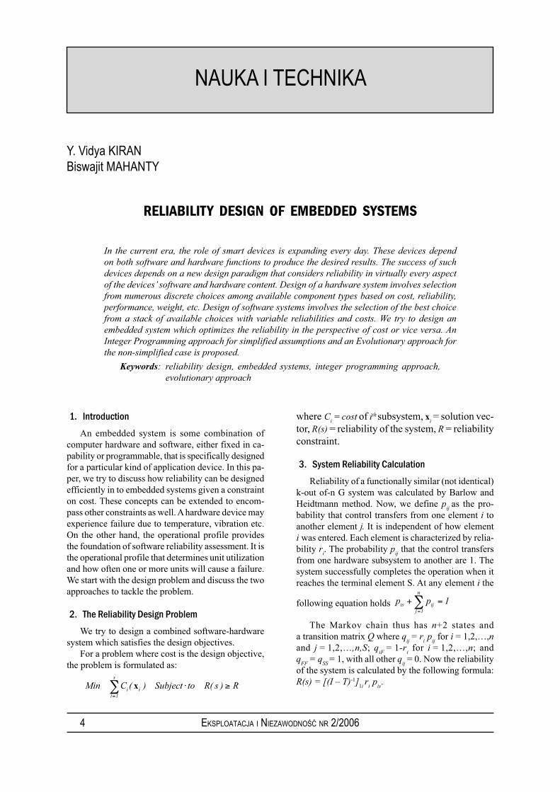
Both the cases have the following transfer probabi-lities. The rectangles represent software modules and the rhombuses represent the hardware elements.
5.1. Test Case 1
This case has the assumptions which we used for integer programming approach. Following are the choices for each element given in the form (Relia-bility, Cost). HW represents Hardware Element and SW means Software module.
1(HW): (0.8,2); 2(HW): (0.9,4); 3(SW): (0.8,2.5), (0.85,3), (0.9, 4), (0.95,5); 4(SW): (0.9,3), (0.95,4.5), (0.98,6); 5(SW): (0.95,3.5), (0.97,5); 6(SW): (0.92,2.5), (0.96,4.0), (0.98,5.5);7(HW): (0.85,5); 8(HW): (0.95,7)
6 EKSPLOATACJA I NIEZAWODNOŚĆ NR 2/2006
NAUKA I TECHNIKA
The constraint in the above problem was taken to be the cost which was not supposed to exceed 55 units. Integer Programming and Genetic Algorithms (with parameters p_mut = 0.05; p_crossover = 0.65, Generations = 400, population = 15) returned the same answer for this deterministically solvable problem. Reliability = 0.757683 Cost = 54.5
5.2. Test Case 2
Following are the choices for each element given in the form (Reliability,Cost)1(HW)-(0.8,2),(0.9,3),(0.95,3.5),(0.97,5);
2(HW)- (0.9,4);(0.92,4.5);(0.97,6)3(SW)- (0.8,2.5), (0.85,3), (0.9, 4), (0.95,5); 4(SW)- (0.9,3); (0.95,4.5);(0.98,6)5(SW)-(0.95,3.5), (0.97,5);
6(SW)-(0.92,2.5), (0.96,4.0), (0.98,5.5)7(HW)-(0.85,5), (0.88,6), (0.92,7.5), (0.95,8.5), (0.99,10); 8(HW)-(0.95,7),(0.98,9),(0.99,10.5)
Constraint is that the Reliability of the system should be greater than 0.8
Genetic Algorithms produced the following result: Reliability = 0.800576 Cost = 57.5; p_mut = 0.05; p_crossover = 0.65; Genera-tions = 400, population = 15
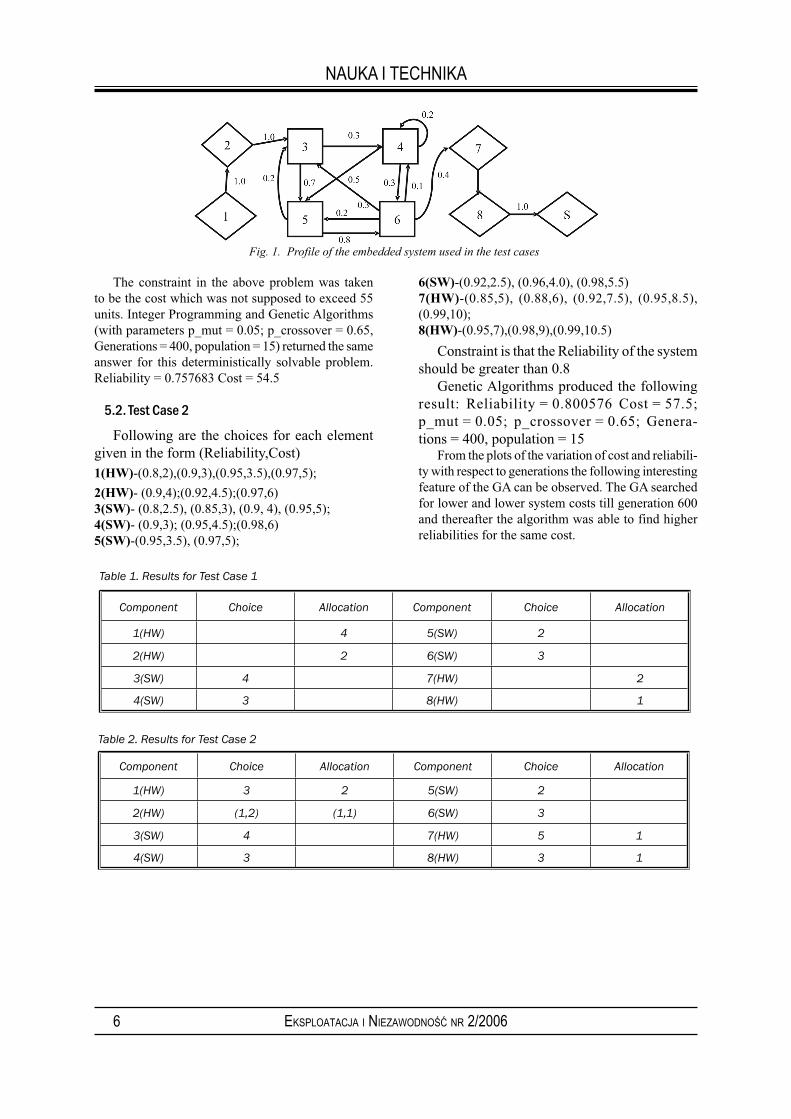
From the plots of the variation of cost and reliabili-ty with respect to generations the following interesting feature of the GA can be observed. The GA searched for lower and lower system costs till generation 600 and thereafter the algorithm was able to find higher reliabilities for the same cost.
Fig. 1. Profile of the embedded system used in the test cases
Component Choice Allocation Component Choice Allocation
1(HW) 4 5(SW) 2
2(HW) 2 6(SW) 3
3(SW) 4 7(HW) 2
4(SW) 3 8(HW) 1
Table 1. Results for Test Case 1
Component Choice Allocation Component Choice Allocation
1(HW) 3 2 5(SW) 2
2(HW) (1,2) (1,1) 6(SW) 3
3(SW) 4 7(HW) 5 1
4(SW) 3 8(HW) 3 1
Table 2. Results for Test Case 2
7EKSPLOATACJA I NIEZAWODNOŚĆ NR 2/2006
NAUKA I TECHNIKA
6. Conclusions
The design problem was successfully tackled with the two approaches discussed. The results are very promising with proven optimal convergence on a sim-
7. References
[1] Barlow, R. E. and K. D. Heidtmann (1984). Computing k-out-of-n system reliability. IEEE Trans. Reliability. R-33, 322–323.
[2] Siegrist, K. (1988). Reliability of Systems with Markov Transfer of Control. IEEE Transactions on Software Engineering. 14, 1049-1053.
[3] Misra, K. B. and U. Sharma (1991). An efficient algorithm to solve integer programming problems
arising in system reliability design, IEEE Transactions on Reliability, 40, 81-91.[4] Smith, A. E. and D. M. Tate (1993). Genetic optimization using a penalty function. Proceedings of
the 5th International Conference on Genetic Algorithms, 499-505.
plified problem wherein both the approaches give the same optimal results. The GA approach has a probable near-optimal convergence on the complex problem too. Future work may be directed at solving the design problem with more realistic assumptions.
Ing. Y. Vidya KIRAN Dr. Prof. Biswajit MAHANTY
Department of Industrial Engineering and ManagementIndian Institute of TechnologyKharagpur (W.B) 721 302, Indiae-mail: [email protected]: [email protected]
Fig. 2. Cost and Reliability Variation with Generations

8 EKSPLOATACJA I NIEZAWODNOŚĆ NR 2/2006
Kailash C. KAPUR
MULTI-STATE RELIABILITY: MODELS AND APPLICATIONS
This paper focuses on customer-centered reliability models and measures for multi-state sys-
tems with multi-state components. A review of general models which capture the customer’s
experience with the product is presented. An approach is given to develop the system structure
function using equivalent classes and develop reliability bonds. In addition to measures and
models, ideas are given for potential applications of these models to infrastructure problems
such as transportation, computer network, supply chain, communication systems and network
reliability.
Keywords: Multi-state reliability, multi-state systems and components, general struc-
ture functions, reliability bounds
1. Introduction
In the traditional reliability methods (Kapur et al. 1997), the system and all of its components are assumed to have only two states of working effi-ciency which are working perfectly and total failure. Although this assumption simplifies the complicated problems for reliability evaluation, it losses the ability to reflect the reality that most systems actually degrade gradually and have a wide range of working efficiency (Barlow et al. 1978, Boedigheimer et al. 1994, Kapur 1986, Lisnianski et al. 2003, and Natvig 1982). In the literature most of the work on multi-state reliability research makes the assumption that the system and all of its components have same number of states. This assumption is not realistic because in reality the system and components have different numbers of sta-tes (Lisnianski et al. 2003, Boedigheimer et al. 1994, Brunelle et al. 1997 and 1999, Hudson et al., 1983 and 1985). The main focus of this paper is to make sure that the reliability measures capture the reality of multiple states for the systems and the components, and assure that they can capture the total experien-ce of the customer with the system. Then these general measures can be applied to broad problems in engineering systems, supply chain and logistics, general networks for transportation and distribution, and computer and communication systems.
2. Development of general structure function
For a multi-state system with n components, let each component i have (m
i+1) different and distinct
states or levels of working efficiency. Also the system has M+1 different levels of working efficiency.
Let S = [0, 1, …, m1] × [0, 1, …, m
2] × … × [0, 1, …,
mn] be the components state space, and s = [0, 1, …, M]
be the set of all possible states of the system. Then we
can express the relationship between the components and system at time t by
For any state of working efficiency k ∈ (0, 1, …, M) of a system, we define
where x = (x1, x
2, ... , x
n)
Sk is known as the Equivalent Class, the collection of
all combination of the n components with different states that make the system to be in state k. S
k’s are
mutually exclusive and , the component state space. Let Ө
k be the number of elements in each
S k. Of those Ө
k different elements, L
k of them are cal-
led the “Lower Boundary Points” and Uk of them are
called the “Upper Boundary Points”.
Definition 1 (Lower Boundary Points):
x = (x1, x
2, ... , x
n) ∈ S
k is called a lower boundary
point if only if for any y = (y1, y
2, ... , y
n) < x, then
.
Definition 2 (Upper Boundary Points):
x = (x1, x
2, ... , x
n) ∈ S
k is called an upper boundary
point if only if for any y = (y1, y
2, ... , y
n) > x, then
.
is called the “Lower Boundary Points Set” and is the i
th
lower boundary point for Sk, .
is called the “Upper Boundary Points Set” and is the i
th
upper boundary point for Sk, .

9EKSPLOATACJA I NIEZAWODNOŚĆ NR 2/2006
NAUKA I TECHNIKA
2.1. Generation of the generic structure function with
lower (upper) boundary points
With the lower boundary points ( ), Liu et al. (2004) have developed the generic structure function for the system. From the definition of the lower boundary point, we know that a system is in the state k or higher if x is greater than or equal to at least one lower boundary point in the lower boundary points set LB(k). We can formulate this as
If then let . When k = 0 means that the system is totally failed, and we
let Then the structure function is
Similarly, with the upper boundary points ( ), we can formulate
If then let . When k = M means that the system is perfectly working, and M
we let Then the structure function is
Using the above structure functions, we can find the expected values of the state of the system as below:
and
2.2. Reliability bounds
In addition, we can find bounds on the expected values of state of the system as below (for details see Liu et al. (2004)).
The lower bound is
and the upper bound is
2.3. Example
Consider a system with two components with m
1 = 3, m
2 = 2 and M = 3. The information on the bo-
undary points is given in Table1, and information for the component state probabilities is given in Table2.
For this system, we get using either the lower boundary points or upper boun-dary points. Also, bounds on system reliability are
.
3. Customer-centered reliability measures
One proposed measure for customer-centered reliability for a target life t
0 is
With customer's utility as a function of the state of the system, we can calculate the customer's expected total utility for experience (ETUE) with the system from time 0 to time t
0. This is given by:
The greater the ETUE, the better the system is for the customer.
For details and applications of these measures, see [Liu et al. 2005].
k Sk
Lower Boundary Point Upper Boundary Point
0 (0,0) (0,0)1 (3,0),(2,0),(0,2),(1,0),(0,1) (1,0),(0,1) (3,0),(0,2)2 (2,2),(3,1),(2,1),(1,2),(1,1) (1,1) (2,2),(3,1)3 (3,2) (3,2)
Table 1. Lower/Upper Boundary Points
Component Component State (x)
0 1 2 3
1 0.2 0.4 0.1 0.3
2 0.3 0.2 0.5
Table 2. Component-state Probability

10 EKSPLOATACJA I NIEZAWODNOŚĆ NR 2/2006
NAUKA I TECHNIKA
4. Infrastructure applications
Modern society increasingly relies on infrastructu-re networks such as supply chain and logistics, trans-portation networks, commodity distribution networks (oil/ water/ gas distribution networks), computer and communication networks, etc. Network and its com-ponents can provide several levels of performance and thus the performance of the network and its com-ponents can be considered as a range from perfect functioning to complete failure.
A network consists of two classes of components: nodes and arcs (or edges). A topology of a network model can be represented by a graph, G = (N, A) where N ={s, 1, 2,…, n, t} is the set of nodes with s as the source node and t as the sink node and A = {a
i|1 ≤ i ≤ n} is the set of arcs where an arc a
i
joins an ordered pairs of nodes (i, i')∈ N× N such that i ≠ i'. Let m = {m
1, m
2, …, m
n} be a vector of maximum
capacities for the arcs. Assume all the nodes in the network are perfectly reliable. Based on the maximum capacity, we can easily find the maximum flow in the
network from node s to node t. This maximum value of flow is equivalent to state M of the system for the development of the structure function in section 2, and 0 ≤ k ≤ M. The actual capacity at any time of the arc degrades from m
i, i = 1, …, n, to 0. Let x
i be the actual
capacity of the arc ai, 0 ≤ x
i ≤ m
i, and x
i integer.
We can solve the following optimization problem:
Max f
subject to
Ext = (es - e
t) f, E is the node-arc incidence matrix
xt ≤ mt
xt ≥ 0 and integer.
Thus, , the equivalent class for the highest value M of the state of the system.
Research is under way to generate all the equivalent classes and their boundary points. Then we can apply the methods discussed in sections 2 and 3 to evaluate reliability of the infrastructure networks.
5. References
[1] Barlow, R.E. and Wu, A.S. (1978). Coherent Systems with Multistate Components, Mathematics of Operations Research, Vol. 3, No. 4, 275-281.
[2] Boedigheimer, R., and Kapur, K.C. (1994). Customer Driven Reliability Models for Multistate Coherent
Systems, IEEE Transactions on Reliability, Vol. 43, No. 1, 46-50. [3] Brunelle, R.D. and Kapur, K.C. (1999), Review and Classification of Reliability Measures for Multistate and
Continuum Models, IIE Transactions, Vol. 31, No. 12, 1171-1180. [4] Brunelle, R.D. and Kapur, K.C. (1997). Customer-Center Reliability Methodology, In: Proceedings of the
Annual Reliability and Maintainability Symposium, 286-292. [5] Hudson, J.C. and Kapur, K.C. (1983). Reliability Analysis for Multistate Systems with Multistate Components,
IIE Transactions, Vol. 15, No. 2, 127-135. [6] Hudson, J.C. and Kapur, K.C. (1985). Reliability Bounds for Multistate Systems with Multistate Components,
Operation Research, Vol. 33, No. 1, 153-160. [7] Kapur, K.C., and Lamberson, L.R. (1977). Reliability in Engineering Design, John Wiley, New York. [8] Kapur, K.C. (1986). Quality Evaluation Systems for Reliability, Reliability Review, Vol. 6, No 2. [9] Lisnianski, A., and Levitin, G. (2003). Multi-state System Reliability: Assessment, Optimization and Applications,
World Scientific Pub. Co., Inc.[10] Liu, Y. and Kapur, K.C. (2004, October). Structure Function and Reliability Bounds for Generalized Multi-
state Components, Technical Report, Industrial Engineering, University of Washington, Seattle.[11] Liu, Y. and Kapur, K.C. (2005, February 15-17). Stochastic Customer-Centered Measures for Multi- state
Reliability, In: Proceedings of Stochastic Models in Reliability, Safety, Security and Logistics, Israel.[12] Natvig, B. (1982), Two Suggestions of How to Define a Multistate Coherent System, Adv. Applied Probability,
Vol. 14, 434-455.
Kailash C. KAPUR
Industrial Engineering, University of WashingtonBox 352650, Seattle, WA 98195-2650, USAe-mail: [email protected]

11EKSPLOATACJA I NIEZAWODNOŚĆ NR 2/2006
Milan HOLICKÝ
FUZZY PROBABILISTIC MODELS IN STRUCTURAL RELIABILITY
Two types of uncertainties can be generally recognised in structural reliability: natural ran-
domness of basic variables and vagueness of performance requirements. While the randomness
of basic variables is handled by common methods of the probability theory, the vagueness of
the performance requirements is described by the basic tools of the theory of fuzzy sets. Both
the types of uncertainties are combined in the newly defined fuzzy probabilistic measures of
structural reliability, the damage function and the fuzzy probability of failure. The proposed
measures can be efficiently applied in a similar way as conventional probabilistic quantities for
the verification and optimisation of structural reliability. Adequate data are however needed
for further development of the outlined concepts.
Keywords: structural reliability, fuzzy probabilistic measures, damage function
1. Introduction
The performance requirements (serviceability constraints, structural resistance) of buildings and engineering works are often affected by various un-certainties that can hardly be described by traditional probabilistic models. As a rule, the transformation of human desires, particularly of those describing occupancy comfort and aesthetical aspects, to per-formance requirements often results in an indistinct or imprecise specification of the technical criteria for relevant performance indicators (for example permis-sible deflection, acceleration). Thus, in addition to the natural randomness of basic variables, the perfor-mance requirements may be affected by vagueness in the definition of technical criteria. Two types of the uncertainty of performance requirements are identi-fied here: randomness, handled by commonly used methods of the theory of probability, and fuzziness, described by the basic tools of the theory of fuzzy sets (Brown 1983, Shiraishi 1983). Similarly as in the previous studies (Holický 1993, 1996 and 2001), the performance condition S ≤ R, relating an action effect S and a relevant performance requirement R, is analysed assuming the randomness of S and both the randomness and the fuzziness of R.
2. Fuzzy probabilistic models of performance requ-
irements
Fuzziness due to vagueness and imprecision in the definition of performance requirement R is de-scribed by the membership function ν
R(x) indicating
the degree of the membership of a structure in a fuzzy set of damaged (unserviceable) structures (Holický 1993, 1996 and 2001); here x denotes a generic point of a relevant performance indicator (a deflection or a root mean square of acceleration) considered when assessing structural performance. A common
experience indicates that a structure is loosing its ability to comply with specified requirements gradu-ally within a certain transition interval <r
1, r
2>. The
membership function νR(x) describes the degree of
structural damage (lack of functionality). If the rate dν
R(x)/dx of the “performance damage” in the interval
<r1, r
2> is constant (a conceivable assumption), then
the membership function νR(x) has a piecewise linear
form as shown in Figure 1. It should be emphasized that ν
R(x) describes the non-random (deterministic)
part of uncertainty in the requirement R related to economic and other consequences of inadequate per-formance. The randomness of R at any damage level ν = ν
R(x) may be described by the probability density
function φR(x|ν) (see Figure 1), for which the normal
distribution having a constant standard deviation σν
is considered here.
The transition region < r1 , r
2 >, where the structure
is gradually losing its ability to perform adequately and its damage increases, may be rather broad depend-ing on the nature of the performance requirement. For
Fig. 1. The fuzzy probabilistic model of the performance
requirement R

12 EKSPLOATACJA I NIEZAWODNOŚĆ NR 2/2006
NAUKA I TECHNIKA
common serviceability requirements (deflections) the upper limit r
2 may be a multiple of the lower limit r
1
(for example r2 = 2 r
1). An extreme example is the
case of continuous vibration in buildings specified in the International Standards (ISO 1989 and 1991) and discussed by Bachmann (1987) (see also a previous study by Holický (1996)). In general the acceleration constraints for continuous vibration are considered within a range from 0.02 to 0.06 ms-2. There is a low probability of an adverse comment for accelerations below the lower limit r
1 = 0.02 ms-2. On the other hand
adverse comments are almost certainly expected for accelerations above the upper limit r
2 = 0.10 ms-2, thus,
in that case r2 = 5 r
1.
3. Fuzzy probabilistic measures of structural perfor-
mance
The damage function ΦR(x) is defined as the
weighted average of damage probabilities redu-ced by the corresponding damage level (Holický 1993, 1996 and 2001)
(1)
where N denotes a factor normalising the damage function Φ
R(x) to the conventional interval <0, 1>
(see Figure 1) and is a generic point of x. The damage function Φ
R(x) defined by equation (1) may be con-
sidered as a generalised distribution function of the performance requirements R that can be used for the specification of the design (or characteristic) value of the requirements R corresponding to a given level of the total expected damage. The density of the damage φ
R(x) follows from (1) as
(2)
Figure 2 shows variation of the statistical pa-rameters of the performance requirement R with σ
v /(r
2 − r
1). It appears that Beta distribution with
the origin at zero can be used as an approximation of φ
R(x). If the standard deviation σ
v = 0.2 (r
2 − r
1),
then μR = r
1+ 0.67(r
2 − r
1), σ
R = 0.31(r
2 − r
1) and
σR
= − 0.25, Beta distribution has the bounds a = 0, b = r
1+1.65(r
2 − r
1) and the shape parameters c = 10.07
and d = 5.88. The fuzzy probability of performance failure π can
be defined provided that the probability density func-tion of the action effect S, denoted φ
S(x) is known as
π = (3)
An asymmetric three parameter lognormal distribution of S is accepted in earlier studies (Holický 1993, 1996 and 2001). The damage func-tion Φ
R(x) defined by equation (1) and the fuzzy
probability of performance failure π defined by equation (3) enable the formulation of various de-sign criteria in terms of relevant randomness and fuzziness parameters. However, adequate data for the specification of the fuzziness parameters r
1,
r2, the membership function v
R(x) and its standard
deviation σv (describing the requirement R), the
probability density φS(x) of the load effect S and
its characteristics are needed.
4. Optimisation
The optimum value of the fuzzy probability of performance failure can be estimated using the technique of design optimisation (Holický 1996 and 2001). It is assumed that the objective function is given by the total cost C(ξ) expressed approximately as the sum
C(ξ) = C0(ξ) + π(ξ) C
D (4)
where C0(ξ) is given as the sum of the construc-
tion and maintenance cost, π(ξ) CD is the expec-
ted malfunction cost; here CD denotes the cost of
full damage (full malfunction or serviceability failure) and ξ denotes the decision parameter (for example the mass per unit length or the cross section area). It has been shown (Holický 1996 and 2001) that this equation can be used if the malfunction cost due to the damage level v is given as the multiple v
R(x)C
D (in the example of
continuous vibration it represents the cost due to disturbance and the lower efficiency of occupan-
Fig. 2. Variation of the statistical parameters of the perfor-
mance requirement R with σν /(r
2−r
1)

13EKSPLOATACJA I NIEZAWODNOŚĆ NR 2/2006
NAUKA I TECHNIKA
cies in the offices). Further, it is assumed that both the initial cost C
0(ξ) and the fuzzy probability of
performance failure π(ξ) are dependent on a de-cision parameter ξ (for example on the mass per unit length of a floor component) while the cost of full damage C
D is independent of ξ. If C
0(ξ)
is proportional to the decision parameter ξ, and the load effect S is proportional to a power ξ−k
(k≥1), then the optimum ratio CD
/C0(ξ) may be
expressed as
(5)
where the quantities C0(ξ), μ
S(ξ), σ
S(ξ) are de-
pendent on the decision parameter ξ. Partial derivatives of the fuzzy probability of failure π in equation (5) are to be determined using equ-ation (3) and numerical methods of integration and derivation. Previous optimisation studies of various structural aspects indicate that common-ly used performance requirements including the
deformation and acceleration constraints may be uneconomical (Holický 1996 and 2001).
5. Concluding remarks
(1) Performance requirements on structural beha-viour are generally affected by two types of uncertainty: randomness and vagueness due to indistinct or imprecise definitions and percep-tion.
(2) The newly developed fuzzy probabilistic con-cepts provide valuable measures enabling the reliability analysis and optimisation of structural performance.
(4) Previous optimisation studies indicate that commonly used performance criteria for servi-ceability constraints concerning deflection and continuous vibration may be uneconomical.
(5) Further development and practical applications of the fuzzy probabilistic concepts require ap-propriate experimental data enabling an adequ-ate specification of initial theoretical models.
Acknowledgement
This study is a part of the research project CEZ: J04/98:210000029 “Reliability and risk engineering of tech-
nological systems “, supported by the Ministry of Youth and Education of the Czech Republic.
6. References
[1] Bachmann, H. and W. Ammann (1987). Vibration in structures induced by man and machines, Zurich: IABSE.
[2] Brown, C.B. and J.T.P. Yao (1983). Fuzzy sets and structural engineering. Journal of structural engineering, 109, 5, 1211-1225.
[3] Holický, M. and L. Őstlund (1983). Probabilistic design concept. In: Proc. International colloquium IABSE: Structural serviceability of buildings, Gőteborg, pp. 91 - 98.
[4] Holický, M. (1996). Fuzzy probabilistic optimisation of building performance. In: Proc. CIB-ASTM-ISO-RILEM International symposium - Application of the performance concept in building, Tel Aviv, 1996, pp. 4-75 to 84. (see also Automation in construction 8, 4, 1999; pp. 437-443).
[5] Holický, M. (2001). Performance deficiency of a department store–case study, In: Proc. Safety, risk and reliability–Trends in engineering. International Conference, Malta 2001; Zürich, IABSE, pp. 321-326.
[6] ISO 2631-2 (1989). Evaluation of human exposure to whole/body vibration - Part 2: Continuous and shock-induced vibration in buildings (1 to 80) Hz.
[7] ISO 10137 (1991). Basis for design of structures - Serviceability of buildings against vibration.[8] Shiraishi, N. and H. Furuta (1983). Structural design as fuzzy decision model. In:Proc. ICASP 4, Pitagora
Editrice, Bologna, p. 741-752.
Prof. Ing. Milan HOLICKÝ, Dr Sc.
Klokner Institute of the Czech Technical University in PragueSolinova 7, 166 08 Praha 6, Czech Republice-mail: [email protected]
14 EKSPLOATACJA I NIEZAWODNOŚĆ NR 2/2006
Rose D. BAKER
RISK AVERSION IN MAINTENANCE
The concept of risk averse maintenance is introduced. It is formulated in terms of seeking to
minimize a disutility rather than a cost per unit time. A general formalism is given, followed
by an example, the application to age-based replacement. The problem of overmaintenance
caused by undue risk aversion on the part of engineers is briefly discussed.
Keywords: risk-aversion, age-based replacement, maintenance, utility-function ap-
proach
1. Introduction
The concept of risk-aversion is central to economic and financial thought. In this context, the word ‘risk’ denotes variability in cash flows. In general, both individuals and organizations are risk averse, and this has implications for maintenance practice. Risk averse policies require more frequent replacement or maintenance. The higher spend on maintenance can be thought of as an insurance against unexpected losses.
There seems to be no existing work on risk-averse maintenance policies, and very little on risk-averse operational research in general. Exceptions are the papers of Padmanabhan and Rao (1993) and Chun and Tang (1995), who have studied risk-averse warranty policies.
In this paper, risk-averse maintenance policies are modelled using the methodology of utility functions developed in economics. Rather than seeking to mini-mize a mean cost per unit time, a rational risk-averse individual would seek to maximize a concave utility function.
A degree of risk aversion is entirely rational. A conflict of interest can however arise when a ma-intenance engineer carries out maintenance policies on behalf of Management. If the engineer is more risk averse than the manager, from the viewpoint of mana-gement, the equipment is being overmaintained. This is an example of what within principal-agent theory (e.g. Laffont and Martimort 2002) is called the moral hazard problem. A solution is to use incentives to induce maintenance engineers not to overmaintain. There is not space to discuss this topic further.
2. Risk-averse maintenance
Risk aversion can be modelled via a concave utility function. The utility of a sum of money y is U(y), where U’ > 0, U” < 0, the primes denoting differentiation.
We use here only the exponential utility function, defined as
(1)
where η > 0 is a measure of risk aversion. An expen-diture x = -y has disutility
(2)
and this form is used from now on. The certainty-equivalent of a policy is the sum of
money that if definitely gained or lost would have the same expected utility as the variable cashflows of the policy. Here we use the certainty equivalent sum D per unit time. Hence if a policy is carried out for time T, we have for the exponential utility function that
or
(3)
Using the exponential utility function given in equation 2, consider a general maintenance or repla-cement policy in which cycles, which can be of fixed or variable length, end in replacement, inspection, or some regenerating event. During the ith cycle, a ran-dom number of failures N
i occurs, at cost c
f each, and
the regenerating event has cost cs. More generally,
a random cashflow Fi occurs during the cycle. Con-
sider the certainty-equivalent expenditure per unit time D, when the cycles continue to some very large time T. We consider first the case where cycles are of fixed length t.
The certainty-equivalent expenditure per unit time is then
15EKSPLOATACJA I NIEZAWODNOŚĆ NR 2/2006
NAUKA I TECHNIKA
Hence as the cycles are independent,
(4)
dropping the cycle subscript i. This is the criterion to be minimized in place of the cost per unit time.
The expression E exp(ηF) is the moment genera-ting function of the random variate F, with parameter η. If F
i = c
f N
i + c
s, then
E exp(ηF) = exp(η cs) E(η c
fN)
i.e. proportional to the mgf. of the number of failures, with parameter c
f η.
For optimization problems the task of finding the mean of a random variate has been replaced by the task of finding its moment generating function. In general, log E exp(ηF) is the cumulant generating function, so that
where κj is the jth cumulant of the cost per cycle. As
risk aversion increases, the function D to be minimised puts increasing weight on the higher cumulants, such as skewness and kurtosis.
When cycles have variable length, such as for age-based replacement, equation 4 becomes
where PN is the probability that N cycles of the em-
bedded renewal process have occurred by time T, and hence G is the moment generating function for the number of cycles. Thus,
(5)
where log G is the cumulant generating function for the number of cycles.
There is an elegant exact solution for D, from applying the Wald identity to a renewal process (Cox 1962). This identity yields the asymptotic result
log Eexp(-logM(s)N(T)) = sT (6)
where M(s) = E(exp(-st)), and the expectation is of the distribution of cycle length. The left hand side of equation 6 is the cumulant generating function of the number of cycles N(T). Hence equation 5 yields simply
(7)
where is the value of s for which the coefficient of N(T) in equation 6, equals log Eexp(ηF), i.e.
(8)
The exact calculation of D from equation 7 requires
only the solution of equation 8 for , or explicitly
(9)
where S(u) is the survival function of the cycle length. This equation can be solved by Newton-Raphson ite-ration.
As an example, in age-based replacement an item is replaced at age t or on failure. The cost per unit time is
where S(t) is the survival function of the failure-time distribution (Jardine, 1973).
Let X be a random (indicator) variable, where X = 1 denotes failure in (0, t] and X = 0 denotes su-rvival to time t without failure. Then
where .
Expanding the exponential, since X is idempotent and E(X) = 1 – S(t),
and rearranging
(10)
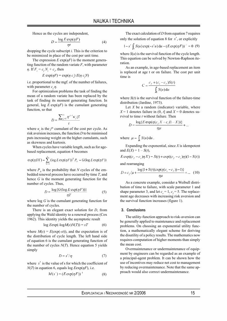
As a concrete example, consider a Weibull distri-bution of time to failure, with scale parameter 1 and shape parameter 3, and let c
s = 1, c
f = 5. The replace-
ment age decreases with increasing risk aversion and the survival function increases (figure 1).
3. Conclusions
The utility-function approach to risk-aversion can be generally applied to maintenance and replacement problems. On choosing an exponential utility func-tion, a mathematically elegant scheme for deriving the disutility of a policy results. The mathematics now requires computation of higher moments than simply the mean cost.
Overmaintenance or undermaintenance of equip-ment by engineers can be regarded as an example of a principal-agent problem. It can be shown how the use of incentives may reduce net cost to management by reducing overmaintenance. Note that the same ap-proach would also correct undermaintenance.

16 EKSPLOATACJA I NIEZAWODNOŚĆ NR 2/2006
NAUKA I TECHNIKA
This general approach to risk aversion could be used throughout OR, wherever a minimum cost per unit time policy is considered. As human beings are undoubtedly risk-averse, it is a little surprising that
Fig. 1. Age based replacement with a Weibull distribution of scale parameter
1, shape parameter 3, replacement cost cs = 1, failure cost c
f = 5.
The solid line shows the variation of optimum age at replacement
with the risk-aversion parameter η, and the dotted line the survival
function
4. References
[1] Chun, H.C and K.Tang (1995). Determining the optimal warranty price based on the producer’s and customers’
risk preferences. European Journal of Operational Research, 97-110. [2] Cox, D.R. (1962). Renewal Theory. London: Chapman and Hall. [3] Jardine, A.K.S. (1973). Maintenance, Replacement and Reliability. Pitman, Bath. [4] Laffont, J.J. and D. Martimort (2002). The theory of incentives: the principal-agent model. Princeton:
Princeton University Press. [5] Padmanabhan, V. and R.C. Rao (1993). Warranty policy and extended service contracts: theory and an
application to automobiles, Marketing Science, 230-247.
Dr. Prof. Rose D. BAKER
Centre for Operational Research and Applied Statistics University of Salford, UKe-mail: [email protected]
OR routinely ignores this fact. Modifying standard OR solutions to include risk aversion gives a wide application area indeed.

17EKSPLOATACJA I NIEZAWODNOŚĆ NR 2/2006
Igor A. USHAKOV
TERRESTRIAL MAINTENANCE SYSTEM FOR GEOGRAPHICALLY DISTRIBU-
TED CLIENTS
Clients (for instance, owners of ground equipment for satellite telecommunication network)
are arbitrarily distributed on some territory. For maintenance/repair service, one uses Mobile
Maintenance Stations (MMS) located at some Maintenance Bases (MB). The problem is to
construct such maintenance zones which need minimum total number of MMS under condition
that the Quality of Service (QoS) is not worse than required.
A heuristic mathematical model of optimal zoning is suggested. An illustrative numerical example
of constructing service zone for Florida State (USA) is given.
Keywords: maintenance/repair service, maintenance zones, Mobile Maintenance
Stations, Geographically Distributed Clients
1. Brief description of the analyzed system
Assume that clients are arbitrarily distributed wi-thin some territory. Each client possesses equipment, for instance, a dish for receiving satellite signals. After the equipment failure, a client calls to a Maintenance Base (MB) and a Mobile Maintenance Station (MMS) is sent to serve client’s request. If at the moment all MMS are busy then a current client has to wait until any MMS will be free to start moving to the waiting client. For the sake of simplicity, we assume that MMS always start to move to a client from the MB site.
The problem is to construct such zones that the total number of MMS on entire territory is minimum under condition that Quality of Service (QoS) is requ-ired. We will characterize the QoS by two indices: (1) client’s waiting time of response from MB that MMS is directed for service, and (2) namely service time, which includes travel time from MB to the client site and time of repair/maintenance.
Let us give some qualitative arguments about exi-stence of optimal solution of the problem. If the zone radius is chosen too small, it will be enough a single MMS within the zone. In this case, the number of service zones is huge, and for each zone, an adequate mathematical model will be M/G/1 queuing system. A moderate increase of the zone radius leads to de-crease of the total number of MMS due to the well known fact that queuing system M/G/n with input of nλ is more effective than n systems M/G/1 each with input λ. However, with the radius increase, the average total service time will significantly increase, and, actually, if the radius becomes larger than some value, it will be impossible to conduct maintenance service with required QoS at all.
2. Service zone with a single MMS
2.1. Maximum size of the zone
If call rate per square is low, the zone size (radius) is defined by the physical ability to reach a client for an admissible travel time. For instance, if service time equals 2 hrs, then for 8-hour working day, one has not more than 6 hours for round trip travel, even if the service starts in the very morning. (A factual working day usually is not defined in such strict terms, howe-ver, for the sake of simplicity of the solution, we will not take it into account.) If the average MMS speed is 35mph, then the radius of a service zone will be about 100 miles to satisfy the QoS for a remote client.
Speaking about a zone with low call rate, we keep in mind that the probability of appearance more than one request per a day is low enough (see Fig.1).
Fig 1. Service zone with a single MMS
Of course, if the request is obtained in the middle or at the end of the working day, it can be served only for some nearest clients. For remote clients service is postponed to the next day.

18 EKSPLOATACJA I NIEZAWODNOŚĆ NR 2/2006
NAUKA I TECHNIKA
2.2. Queuing Model for a zone with a single MMS
Let Λ be a call rate within a zone, μ be a service rate, which is defined like:
.
Then MMS can be described by queuing model of type M/M/1. From Queuing Theory (Gnedenko and Kovalenko 1989), one knows that the mean waiting time in such a system is:
(1)
Notice that call rate, Λ, and service rate, μ, depend on service zone radius, r:
Λ (r)=λS (2)
where λ = call rate per sq. mile, S=zone square, and
(3)
where τ = mean repair time, r = zone radius, v = MMS velocity. Resulting expression for the waiting time can be written as:
(4)
where α is some corrective coefficient depending on MB location within the service zone (in practical problems MB locates not I the center of the service zone but At some site with dense population).
3. Service zone with multiple MMS
Assume that it is not enough a single MMS for service all clients within the 100-mile zone. It me-ans that the number of MMS should be increased (Fig.2).
Fig. 2. Service zone with multiple MMS
In this case, an adequate mathematical model is queuing system М/М/n with service discipline FIFO. The mean waiting time can be written as:
(5)
where ρ = the so-called loading coefficient and
(6)
is the stationary probability that multi channel queuing system is not busy at all.
4. Construction of service zones
4.1. Brief description of the method
The suggested procedure is multi-step iterative procedure of finding a “current optimal” location and configuration of service zone. At each step of the procedure, one expands the service zone, and check QoS requirements. At each step, a current decision should be done with taking into account the results obtained at the previous step. In general terms, the procedure might be described as follows:
(1) Construct isolated optimal zone for an MB with a single MMS.
(2) Construct adjacent (neighbor) isolated optimal zone.
(3) Check if it is possible to aggregate these two zones into one with 2 MMS taking into account required QoS (namely, the service time).
(4) Construct the next adjacent zone. This zone expansion should such that allows the zone to be more or less spherical shape.
(5) Repeat the procedure from Step 3. Keep in mind that new aggregation might lead to a necessity of more than two MMS.
(6) Finishing constructing a zone, start to construct the next zone.
(7) Continue the procedure until service zones will cover entire territory.
Notice that the goal function for this optimization problem is multimode, i.e. the resulting solution might essentially depend on the initial “point of growth”.
4.2. Constructing service zones with multiple MMS
Let us consider a situation, when some territory already has been covered with several service zones with a single MMS (Fig.3). Assume that a n aggregate zone with maximum admissible radius can cover all these zones. In this case, we can construct a zone with multiple MMS (Fig.4).
Notice that, as a rule, the number of MMS in the aggregated zone can be decreased.

19EKSPLOATACJA I NIEZAWODNOŚĆ NR 2/2006
NAUKA I TECHNIKA
4.3. Comparison of service zone with a single MMS with
aggregated zone with multiple MMS
Coverage of the territory by an aggregated service zone is more effective than use several zones with a single MMS. Below a comparison of several cases is given.
Fig. 5. Comparison of a group of adjusted individual zones
with an equivalent aggregated zone
Numerical results for several different loading parameters are given in Table 1. The radius of an in-dividual zone with a single MMS is assumed 35 miles (travel time = 1 hour). The radius of the aggregated zone is 105 miles (travel time = 3 hour). The number of MMS for individual zones is always equal to 7.
Naturally, the total loading for the aggregated zone is taken 7 times larger. From the comparison, one can see that for ρ = 0.7 the aggregate service zone decrease
the mean waiting time on 35% and, at the same time, the number of MMS decreases on 14% (6 MMS inste-ad of 7). For ρ = 0.99, one should use 8 MMS and the mean waiting time becomes 3.2 hours but individual zones in this case do not work at all.
5. Case study (Zoning in Florida, USA)
We considered constructing service zones for user’s equipment of a commercial satellite network in Florida (USA). The state is divided onto counties. Each service zone should include or expel entire county.
5.1. Input data
Real statistical data about call rates for different counties were used for constructing service zones. Squares of counties were taken from USA Atlas1. Corresponding input data for the numerical example are given in Table 2. We do not give data for all Flo-rida counties, demonstrating the process only on the Southern part of the state.
The QoS requirements are as follows: (1) the mean waiting time is to be less than 2 hours; (2) travel time is to be less than 3 hours.
5.2. Constructing a first service zone with a single MMS
Step 1. Dade is the first County chosen as initial for the further procedure (it is shadowed by dark gray in Fig. 6). The table with corresponding calculated results us given below.
Fig. 3. Adjusted zones with a single MMS each
Fig. 4. Aggregated zone with multiple MMS
Table 1. Comparison of the mean waiting time
Individual zones Aggregated zoneρ Waiting time # MMS 7ρ Waiting time # MMS
0.7 3.7 hr. 7 4.9 2.5 hr. 60.8 5.1 hr. 7 5.6 1.8 hr. 70.9 9.1 hr. 7 6.3 5.1 hr. 7
0.99 - 7 ≈7 3.2 hr. 8
Table 2. Example of input data for Florida counties
County name Square (sq. miles) Call rate (1/h)
Broward 1211 0,054
Collier 1994 0,010
Dade 1955 0,047
Hendry 1163 0,001
Martin 555 0,005
Monroe 1034 0,005
Palm Beach 1993 0,056
… … …
1 http://www.freac.fsu.edu/InteractiveCountyAtlas/Atlas.html

20 EKSPLOATACJA I NIEZAWODNOŚĆ NR 2/2006
NAUKA I TECHNIKA
Fig. 6. The first choice is Dade County
From Excel program, which has been specially developed for this study, we find that waiting time = 0.5 hrs. Travel time is calculated by special program taking into account the MB location and population dispersion.
Step 2. Next expansion of the first service zone, we obtain by adding Monroe County (see Fig.7). In this figure, the county chosen at the first step is colored by light gray and the new one is again colored dark gray.
Fig. 7. First expansion: county Monroe is added
Calculation of travel time is performed by special sub-program, based on the Manhattan’s metric that gives a possibility to take into account real road ne-twork configuration. From Excel program, we find that for this expanded zone is characterized by the mean waiting time = 0.8 hrs.
Step 3. Add adjacent county – Broward (see Fig. 8). As above, all already chosen counties are in light gray color and new one is darker.
Fig. 8. Next expansion: added county is Broward
We assumed that waiting time should not excess 2 hours. Thus, this solution is unacceptable. At the next step, we will try another adjacent county – Collier instead of Broward.
Step 3a (second trial of step 3). At the second trial of step 3, let us add Collier County instead of Broward (Fig. 9).
Table 3. The 1st step of calculations (County Dade with MB at Miami)
Name Call RateMSS
NumberWaiting
TimeArea
Travel Time
LoadingCoefficient
Radius
Dade 0.047 1,955 0.67 0.167 24.9
Result 1 0.5
Table 4. The 2nd step of calculations (Counties Dade and Monroe with MB at Miami)
Name Call RateMSS
NumberWaiting
TimeArea
TravelTime
LoadingCoefficient
Radius
Dade 0.0471 1,955 0.67 0.167 24.9
Monroe 0.0046 1,034 0.48 0.016 18.1
Total 0.0517 1 2,989 0.82 0.182 30.8
Results 0.8
Table 5. The 3rd step of calculations (Counties Dade, Monroe and Broward, same MB)
Name Call RateMSS
NumberWaiting
TimeArea
Traveltime
Loadingcoefficient
Radius
Dade 0.0471 1,955 0.67 0.166 24.9
Monroe 0.0046 1,034 0.48 0.016 18.1
Broward 0.0540 1,211 0.52 0.191 19.6
Total 0.1057 1 4,200 0.98 0.373 36.6
Result 2.3

21EKSPLOATACJA I NIEZAWODNOŚĆ NR 2/2006
NAUKA I TECHNIKA
Fig. 9. Second trial of Step 3: adding Collier County instead
of Broward County
Since the average waiting time is still in acceptable limits, we are trying to add a next adjacent county.
Step 4. At this step, we add Hendry County (see Fig. 10). There were no calls registered in field statistics du-ring the interval of observation, so we use conservative estimate, assuming 1 call, which in our case corresponds to call rate = 0.0008. (This assumption is marked by symbol “*” next to the name of the added county.)
Fig. 10. Step 4: addition of Hendry County to the fi rst
service zone
Step 5. Since the waiting time is still less than 2 ho-urs, the next adjacent county (Gladis) can be added to this service zone (see Fig. 11). There also were no calls registered in field statistics during the interval of observation, as it was with Hendry County, so we do the same assumptions reflected in the Table 8.
Table 6. Results for step 3a.
Name Call RateMSS
NumberWaiting
TimeArea
TravelTime
LoadingCoefficient
Radius
Dade 0.0470 1,955 0.67 0.166 24.9
Monroe 0.0046 1,034 0.48 0.016 18.1
Collier 0.0100 1,994 0.67 0.035 25.2
Total 0.0617 1 4,983 1.06 0.217 39.8
Result 1.1
Table 7. Results for step 4
Name Call RateMSS
NumberWaiting
TimeArea
TravelTime
LoadingCoefficient
Radius
Dade 0.0471 1,955 0.67 0.166 24.9
Monroe 0.0046 1,034 0.48 0.016 18.1
Collier 0.0100 1,994 0.67 0.035 25.2
Hendry* 0.0008 1,163 0.51 0.002 19.2
Total 0.0625 1 6,146 1.18 0.219 44.2
Result 1.3
Table 8. Results for step 4.
Name Call RateMSS
NumberWaiting
TimeArea
TravelTime
LoadingCoefficient
Radius
Dade 0.0471 1,955 0.67 0.166 24.9
Monroe 0.0046 1,034 0.48 0.016 18.1
Collier 0.0100 1,994 0.67 0.035 25.2
Hendry* 0.0008 1,163 0.51 0.002 19.2
Gladis* 0.0008 763 0.63 0.002 16.6
Total 0.0625 1 6,146 1.18 0.223 46.1
Result 1.5

22 EKSPLOATACJA I NIEZAWODNOŚĆ NR 2/2006
NAUKA I TECHNIKA
Fig. 11. Step 4: addition Gladis County to the fi rst service zone
The final solution for the first service zone with a single MMS is presented in Figure 12.
Fig. 12. First service zone
6. Constructing zone with two MMS
In the previous section, we considered only service zones with a single MMS. Here omitting details, we consider the results of constructing of a service zone with two MMS. Notice that actually, in this case, the limiting factor is the permissible travel time.
Fig. 13. Aggregated zone with two MMS.
Suggested method has been used at Hughes Network Systems, Inc. (USA). Evaluated amount of saved money exceeds $3,000,000.
Table 10. Results for service zone with two MMS.
Name Call RateMSS
NumberWaiting
TimeArea
TravelTime
LoadingCoefficient
Radius
Dade 0.0471 1,955 1.11 0.223573 24.9
Monroe 0.0046 1,034 0.81 0.021991 18.1
Broward 0.0540 1,211 0.87 0.256559 19.6
Collier 0.0100 1,994 1.12 0.047647 25.2
Palm Beach 0.0563 1,993 1.12 0.267554 25.2
Hendry* 0.0008 1,163 0.86 0.003665 19.2
Martin 0.0054 555 0.59 0.025656 13.3
Lee 0.0108 803 0.71 0.051 16
Glades* 0.0008 763 0.69 0.004 15.6
St. Lucie 0.0023 581 0.6 0.010 13.6
Charlotte* 0.0008 690 0.66 0.004 14.8
Highlands 0.0023 1,029 0.8 0.011 18.1
Okleehobee* 0.0008 771 0.7 0.004 15.7
Indian River 0.0046 497 0.56 0.022 12.6
Total 0.2006 2 15,039 3.08 0.952 69.2
Results 1.05
7. References
[1] Gnedenko, B.V. and I.N. Kovalenko (1989). Introduction to Queueing Theory. Boston: Birkhauser.[2] Gnedenko, B.V., and I.A. Ushakov (1985). Probabilistic Reliability Engineering. N.Y.: John Wiley &
Sons.
Prof. Ph.D. Igor A. USHAKOV
Editor-in-Chief of Int. e-Journal “Reliability: Theory and Applications”, USAe-mail: [email protected]
23EKSPLOATACJA I NIEZAWODNOŚĆ NR 2/2006
Anatoly LISNIANSKIDavid LAREDOHanoch Ben HAIM
REDUNDANT SYSTEMS SHUTDOWN DURING LOW CAPACITY OPERATION
Two possible operation modes of various pumps with redundancy in electric power generating
units during low load periods (night) were analyzed. The first mode – two of three pumps work
at night with 25% of nominal capacity, the third pump is a cold (passive) reserve. The second
mode – one pump works at night with 50% of nominal capacity, two pumps are in cold reserve.
A Markov reward model was built for the comparison analysis of these possible operation mo-
des. The model takes into account all important factors – pumps power consumption, pumps
failure rate, pumps starting availability, cost of alternative energy, and penalty cost of energy
not supplied. It was shown that under current operation conditions the second operation mode
is more effective one.
Keywords: Auxiliary System, Markov Reward Model, Redundancy, Cold and Hot
Reserve, Mean Accumulated Reward
1. Introduction
Auxiliary systems such as condensing pumps, booster pumps etc are important equipment in pri-mary coal firing generating unit. In present time the operation mode 1 for pumps is used at night during low load period: two of three pumps work at night with 25% of nominal capacity, the third pump is used as passive reserve. In order to decrease electric power consumption the following operation mode 2 was suggested: one pump works at night with 50% of nominal capacity, two pumps are used as passive reserve. The electric power consumption P
2 by the
single pump in the suggested mode 2 is about 66% of the consumption in mode 1. So, the main advantage of mode 2 is the electric power consumption decreasing during low load period. On other hand the using of mode 2 leads to increasing of risk of power generation disturbances because of passive redundant pump may fail to start. The start of reserve pump when working pump failed is provided by control system. If reserve pump failed to start, then the generating power unit will be shut down after short time in order to prevent vacuum breaking. A comparison analysis in order to choice the best operation mode should be based on the measure V =V(1) – V(2), where V(1), V(2) - expected annual cost for operation mode 1 and mode 2 respec-tively. In order to solve this problem a corresponding Markov reward model was suggested.
2. Description of system model
The method is based on the Markov reward model [Hillier and Lieberman, 1995]. This model considers the continuous-time Markov chain with a set of states
{1 ,…, K} and transition intensity matrix a = |aij|, i,
j =1,…,K. It is suggested that if the process stays in any
state i during the time unit, a certain cost rii should be
paid. Each time that the process transits from state i to state j a cost r
ij should be paid. These costs r
ii and r
ij are
called rewards (the reward may also be negative when it characterizes losses or penalties). For such processes, an additional matrix r = | r
ij |, i, j = 1,…,K of rewards
is determined. The value that is of interest is the total expected reward accumulated up to time instant t un-der specified initial conditions. Let V
i(t) be the total
expected reward accumulated up to time t, given the initial state of the process at time instant t = 0 is state i. The following system of differential equations must be solved under specified initial conditions in order to find the total expected rewards:
i =1,…,K. (1)
Usually the system (1) should be solved under initial conditions V
i(0) = 0, i = 1,…,K.
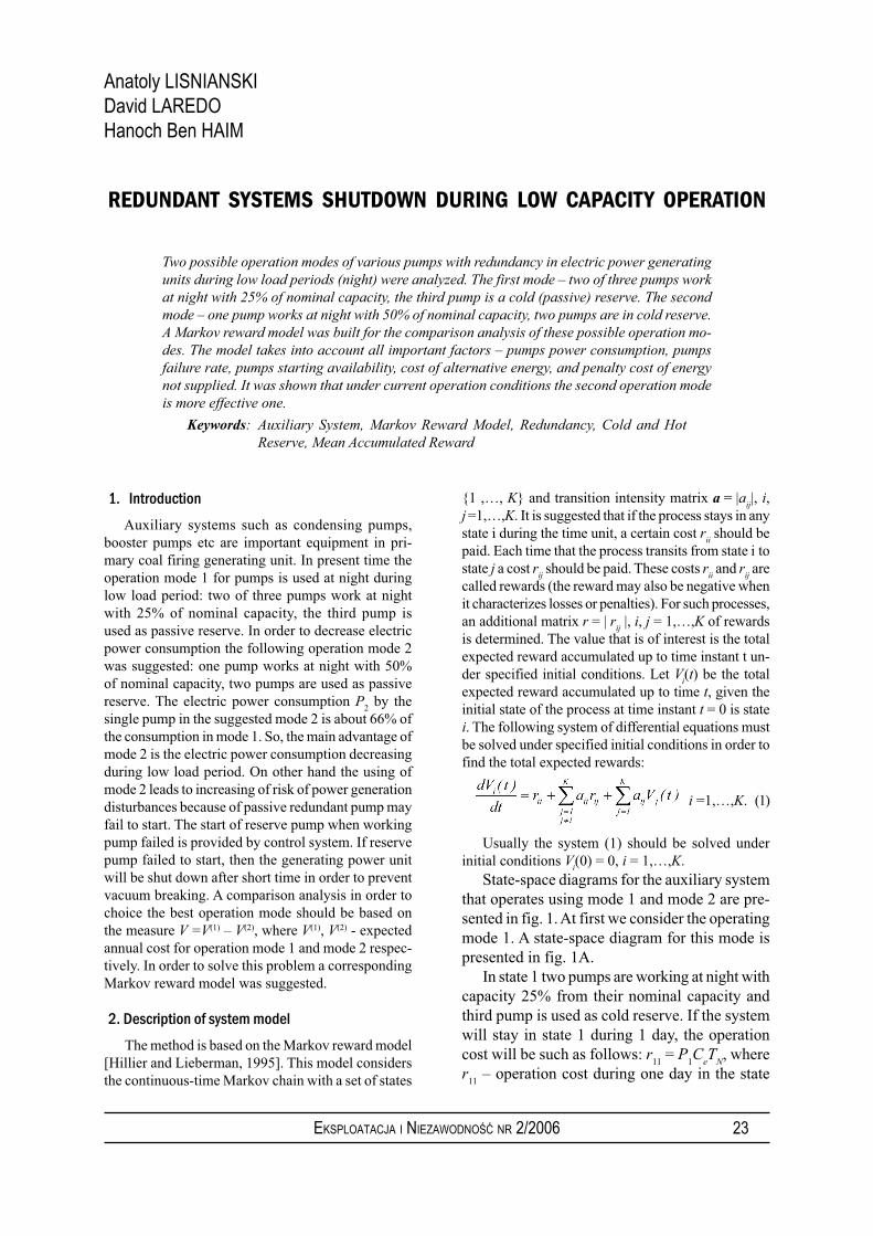
State-space diagrams for the auxiliary system that operates using mode 1 and mode 2 are pre-sented in fig. 1. At first we consider the operating mode 1. A state-space diagram for this mode is presented in fig. 1A.
In state 1 two pumps are working at night with capacity 25% from their nominal capacity and third pump is used as cold reserve. If the system will stay in state 1 during 1 day, the operation cost will be such as follows: r
11 = P
1C
eT
N, where
r11
– operation cost during one day in the state
24 EKSPLOATACJA I NIEZAWODNOŚĆ NR 2/2006
NAUKA I TECHNIKA
1; P1 – electrical power consuming by pumps in
the state 1, when each of two pumps works with capacity 25%; C
e – consumer’s electrical energy
price; TN = 5 hours – low load period (night)
during one day. If one of two pumps working in the state 1 will fail, the system will transit from state 1 to state 2 with intensity rate 2λ, where λ
is a failure rate of one pump. In the state 2 one of reserve pump begins to work and begins a repair of failed pump. We designate by r
22 the operation
cost in state 2. Obviously, r11
= r22
. If a repair of failed pump will be completed before it will be a failure in working pump, the system will come back to state 1 with intensity μ. If an additional failure occurs before than failed pump will be repaired, the system will transit to the state 3 on diagram fig. 1A with transition intensity 2λ. In the state 3 only one pump works with capacity 50% of its nominal capacity and two pumps are under repair. If the system will stay in the state 3 during 1 day, the operation cost will be such as follows: r
33 = P
2C
eT
N, where r
33 – operation cost
during time unit in the state number 3; P2 – elec-
tric power consumption by pump in the state 3, when only one pump works with capacity 50%. In the state 3 two repair teams are working in order to repair both two failed pumps. If repair of one pump will be completed before it will be a failure in the single working pump, than the system will come back to state 2 with intensity rate 2μ. If the single working pump fails before repair will be completed, than the system trans-its from state 3 to state 4 with transition rate λ. The system will be in the state 4 up to trip that prevents a vacuum breaking. In case of vacuum breaking the generating unit is switched off and
a gas turbine starts up. Mean time TL up to trip is
about 30 min. for condensing pumps and about 8 min for booster pumps. Hence, with intensity λ
L = 1/T
L the system will transit from the state 4
to critical state 5. We designate the cost of energy not supplied to consumers that associated with transition from state 4 to state 5 as r
45. This cost
will be the following: r45
= Punit
CpT
st, where P
unit
- generating unit capacity at night (during low load period; C
p - penalty cost for energy not sup-
plied; Tst - time duration of gas-turbines start. In
state 5 gas-turbines begin to work and a cost of alternative energy during the time-unit that au-xiliary system is in the state 5 can be obtained: r
55 = P
unitC
gas, where C
gas is the cost of alternative
energy. In the state 5 the system will be up to the time instant, when a repair of one of the pumps will be completed. In that instant of time the sys-tem transits from the state 5 to the state 3. The intensity of this transition is 3μ.
Fig. 1. State space diagram for auxiliary system operating
in mode 1 (A) and in mode 2 (B).
Hence, the operating mode 1 the system of differential equation (1) can be written in the following form:
(2)

25EKSPLOATACJA I NIEZAWODNOŚĆ NR 2/2006
NAUKA I TECHNIKA
This system should be solved under the fol-lowing initial conditions:
V1(0)=V
2(0)=….=V
5(0)=0.
The expected annual cost for operation mode 1 can be obtained such as V(1) = V
1(t), t = 1 year.
In order to calculate V(2) the Markov reward model for operation mode 2 should be built by the same way. The state space diagram for auxiliary system using operation mode 2 is presented in fig. 1B. The main difference with the previous case is the following. If it will be the failure in the working pump, one of reserve pumps will start by control system. If a control system is available, than reserve pump will start and be-gins to work instead of failed pump. The system transits to state 2 with intensity rate Aλ, where A - control system availability. If a control system is not available, than the system transits from state 1 to state 6 or in state 5 from state 2 with intensity rate (1 – A) λ. In states 5 and 6 operator begins to execute manually control operations in order to start a reserve pump. Mean time for manual pump starting is estimated as T
s = 90 sec.
and therefore, transitions intensity from state 6 to state 2 and from state 5 to state 3 is μ = 1/T
s.
Hence, the following system of differential equ-ations for finding the expected costs V
i(t), i=1,
… , 7 for operation mode 2 can be written (3), where r
11 = P
2C
eT
N, P
2 – electrical power consuming
by pumps in state 1, when only one pump works with capacity 50%. For booster and condensing pumps one has: P
2 = 0.66 P
1.
r33
= r22
= r11
; r47
= r57
= r67
= Punit
CpT
st; r
77 = P
unit G
gas.
As in the previous case the system (3) should be solved under the initial conditions: V
1(0) = V
2(0) =….= V
7(0) = 0. The expected an-
nual cost for operation mode 2 can be obtained such as V(2) = V
1(t), t = 1 year. According to
current data A ≥ 0.99, λ = 1.4 f/y the difference V between expected annual cost for operation mode 1 and mode 2 is estimated as V ≥ 9000 $ per for condensing pumps (for unit with nominal generating capacity 360 MWT) and V ≥ 4000 $ for booster pumps.
3. Conclusions
Operation mode 2 will be preferable and the income from its using instead of mode 1 in power unit with generating capacity 360 MWT will be at least 9000 USA $ per year for condensing pumps and 4000 $ for booster pumps.
(3)
Ph.D. Anatoly LISNIANSKIPh.D. David LAREDOPh.D. Hanoch Ben HAIM
Reliability DepartmentPlanning, Development & Technology DivisionIsrael Electric Corporation Ltd.Str. Nativ Haor 1, Haifa P.O.Box 10, Israele-mail: [email protected]
4. References
[1] Hillier, F. and G. Lieberman (1995). Operations Research. NY, San-Francisco: McGraw-Hill.

26 EKSPLOATACJA I NIEZAWODNOŚĆ NR 2/2006
Radim BRIŠPavel PRAAKS
SIMULATION APPROACH FOR MODELING OF DYNAMIC RELIABILITY
USING TIME DEPENDENT ACYCLIC GRAPH
The dynamic reliability approach takes into account changes (evolution) of the system struc-
ture (hardware). For instance, the dynamic reliability allows modeling a human operator (or
an electronic control system) naturally. In these cases, the structure of the system is usually
changed in order to keep the functionality and/or safety of the system. The main purpose of
the paper is to illustrate, by means of a model example, the ability of acyclic oriented graph,
terminal nodes of which are programmable components, to model simple dynamic system and
to assess its performance via Monte-Carlo simulations. To demonstrate the availability of our
framework a test case study with the deterministic evolution is presented. The here presented
numerical results are in agreement with the exact analytical solution.
Keywords: reliability, complex dynamic systems, oriented acyclic graphs, Monte Carlo
simulation
1. Principles of Dynamic Reliability Approach
One of the main problems in modeling of reliability of complex dynamic systems is to take into account time dependencies of the system structure resulting from changes of its physical parameters. The evolution of the system can be modeled by modifications of values of so called process variables (Pasquet et al., 1998, Labeau, 2000, Chabot et al., 2002). Unfortunately, the traditional modeling techniques see Fig. 1, which are usually based on Boolean modeling, such as Fault Trees and Event Trees, are not suitable for modeling of general dynamic systems because of statistical depend-ency between values of physical parameters and state of components (Chabot et al., 2002). Recently, Neural Networks and Petri Nets approaches were used as tools for reliability analysis of dynamic systems (Pasquet, et. al., 1998, Chabot et al., 2002).
In special cases when times of the structural changes are deterministically scheduled according to a considered time interval, it is possible to solve the problem of reliability assessment. The time partition may be given for example, as a result of evolution of a process variable (Labeau, 2000). The aims of this paper are to present, by means of a P.E. Labeau test-case benchmark demonstrated at ESREL 2002, (i) the efficiency of oriented acyclic graphs (Bris et al., 2002, 2003) to model dynamic systems and (ii) assess their performance using the direct Monte Carlo (MC) simulation technique. Moreover, exactly the same test-case was successfully solved by the Petri Net approach (Chabot et al., 2002).
The structure of this paper is organised as follows. In Section 2, a Dynamic Reliability test-case is de-scribed. Section 3 clarifies ability of acyclic oriented
graphs as a tool for modeling of dynamic systems. Fi-nally, numerical results of MC calculations and future works are presented and discussed in Section 4.
Fig. 1. Traditional Probabilistic Safety Assesment (PSA).
Stochastic character of system inputs is described by
random variables. The output of PSA is a response
of the system, for instance probability of failure. In
contrast of Dynamic Reliability approach, methodo-
logy of PSA assumes that the structure of the system
is constant, non-changing, stable
2. Dynamic Reliability Test-Case Benchmark De-
scription
This example was first proposed by P. E. Labeau. The exact problem description, an analytical solution and an alternative solution can be found at (Labeau, 2000). Let us shortly cite the problem description. For more details, please see (Labeau, 2000) and (Chabot et al., 2002).
“Consider a system (a tank) described by one pro-cess variable x (pressure), with its steady state value x
0. At time t
0, a transient is initiated in state 1, and the
evolution of x follows an exponential law.When the level x = l is reached, a protection device
is solicited (component C1); it can either fail (with

27EKSPLOATACJA I NIEZAWODNOŚĆ NR 2/2006
NAUKA I TECHNIKA
a probability p0), or work correctly (with a probability
1- p0 - p
1, state 2) or be imperfectly triggered (with
a probability p1, state 3). In the last two cases, x starts
to decrease, and a safe shutdown is reached as soon as x < x
0. But if x > L, the system fails (tank rupture).
We add to this description the possibility of an additional component failure (component C
2; λ) that
accelerate the transient, i. e. a transition from state i to i + 3, i = 1, 2, 3.
This more severe transient can still be mitigated in case of a perfect working of the protection device, but it is only slowed down in case of partial triggering. The evolution of x is now as follows:
with a2 > a
3, a
4 = a
1 + b, a
5 = a
2 - b, a
6 = - a
3 + b, and
b > 0. The transition rate is assumed to be constant on [x0, L] and to be 0 outside this range. This makes both final situations (failure and safe shutdown) ab-sorbing”.
Let T be the lifetime of the tank before its rup-ture, i.e., in other words, its failure time. Then the estimation of the probability PL(t) = P(T≤t) is the objective of the calculations carried out via the time dependent acyclic graph model. Following (Labeau, 2000) and (Chabot et al., 2002), we will assume the following numerical values of the parameters of the system, see Tab 1.
Table 1. Parameters of the system
x0
1 p0
0.02 a1
0.2 a4
0.35
l 3 p1
0.04 a2
0.25 a5
0.1
L 4 λ 4.10-2 a3
0.1 a6
0.05
Dynamic reliability approaches suppose the deter-ministic evolution of the process variables, see Fig.2. In other words, we will assume that all changes of hardware configurations are determined (caused) by stochastic events and spontaneous changes of the hardware configuration are not considered (Pasquet et al., 1998).
3. The Time Dependent Acyclic Graph Model
It can be shown that the benchmark has the deter-ministic evolution of the process variable. Moreover, the time partition may be computed analytically. Following (Chabot et al., 2002), we will use the fol-lowing partitioning of the time-interval in the model, see Tab. 2:
Table 2. The time partition of the system mission time
T1 T2 T3 T4 T5 T6
0 3.961 6.931 8.892 11.247 44.205
The continuous evolution of the process variable x(t) and the discrete behaviour of components can be modeled by using the time dependent acyclic graph model, see Figure 3. The model uses the positive logic, so the top event is “Success”. The value in a triangle represents the number of inputs, which must indicate “Success” in order to send the “Suc-cess” to the higher level. Let us shortly describe how the model works. Analyzing Tab.1 and Tab.2, the pro-bability of the non-fail of the component K
1 is [p
0] =
1-p0 = 1-0.02 = 0.998. The component K
2 is modeled
by the shifted exponential distribution with the shift 3.961. This component is switched off (permanent failure) at the time t = 6.931. Farther, the component K
1 is switched off after the time t = 8.892, etc.Consequently (see Figure 3), during the time
interval denoted as a, only corresponding part of the acyclic graph represents the system behaviour. The block inside the dashed box in the same Figure 3, represents the situation “C
2 fails in [0, τ) and C
1 is im-
perfectly triggered”, with τ = 7/3{t - [20 ln 4 - (120/7) ln 3]}. In this case, C
2 is modeled by the component
K3 with the shifted exponential distribution, where
Fig. 2. Three possible states of the process variable in
Dynamic Reliability approach
Fig. 3. The time dependent acyclic graph representation
of the dynamic reliability test-case. Symbols a, b,
c denotes the following time intervals: a = (8.892;
11.247), b = (11.247; 44.205), c = (44.205; ∞)
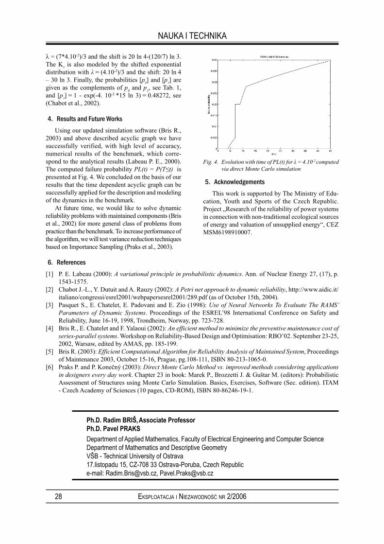
28 EKSPLOATACJA I NIEZAWODNOŚĆ NR 2/2006
NAUKA I TECHNIKA
λ = (7*4.10-2)/3 and the shift is 20 ln 4-(120/7) ln 3. The K
5 is also modeled by the shifted exponential
distribution with λ = (4.10-2)/3 and the shift: 20 ln 4 – 30 ln 3. Finally, the probabilities [p
0] and [p
1] are
given as the complements of p0 and p
1, see Tab. 1,
and [p2] = 1 - exp(-4. 10-2 *15 ln 3) = 0.48272, see
(Chabot et al., 2002).
4. Results and Future Works
Using our updated simulation software (Bris R., 2003) and above described acyclic graph we have successfully verified, with high level of accuracy, numerical results of the benchmark, which corre-spond to the analytical results (Labeau P. E., 2000). The computed failure probability PL(t) = P(T≤t) is presented at Fig. 4. We concluded on the basis of our results that the time dependent acyclic graph can be successfully applied for the description and modeling of the dynamics in the benchmark.
At future time, we would like to solve dynamic reliability problems with maintained components (Bris et al., 2002) for more general class of problems from practice than the benchmark. To increase performance of the algorithm, we will test variance reduction techniques based on Importance Sampling (Praks et al., 2003).
5. Acknowledgements
This work is supported by The Ministry of Edu-cation, Youth and Sports of the Czech Republic. Project „Research of the reliability of power systems in connection with non-traditional ecological sources of energy and valuation of unsupplied energy“, CEZ MSM6198910007.
Fig. 4. Evolution with time of PL(t) for λ = 4.10-2 computed
via direct Monte Carlo simulation
Ph.D. Radim BRIŠ, Associate Professor Ph.D. Pavel PRAKS
Department of Applied Mathematics, Faculty of Electrical Engineering and Computer ScienceDepartment of Mathematics and Descriptive GeometryVŠB - Technical University of Ostrava17.listopadu 15, CZ-708 33 Ostrava-Poruba, Czech Republice-mail: [email protected], [email protected]
6. References
[1] P. E. Labeau (2000): A variational principle in probabilistic dynamics. Ann. of Nuclear Energy 27, (17), p. 1543-1575.
[2] Chabot J.-L., Y. Dutuit and A. Rauzy (2002): A Petri net approach to dynamic reliability, http://www.aidic.it/italiano/congressi/esrel2001/webpapersesrel2001/289.pdf (as of October 15th, 2004).
[3] Pasquet S., E. Chatelet, E. Padovani and E. Zio (1998): Use of Neural Networks To Evaluate The RAMS’
Parameters of Dynamic Systems. Proceedings of the ESREL’98 International Conference on Safety and Reliability, June 16-19, 1998, Trondheim, Norway, pp. 723-728.
[4] Bris R., E. Chatelet and F. Yalaoui (2002): An efficient method to minimize the preventive maintenance cost of
series-parallel systems. Workshop on Reliability-Based Design and Optimisation: RBO’02. September 23-25, 2002, Warsaw, edited by AMAS, pp. 185-199.
[5] Bris R. (2003): Efficient Computational Algorithm for Reliability Analysis of Maintained System, Proceedings of Maintenance 2003, October 15-16, Prague, pg.108-111, ISBN 80-213-1065-0.
[6] Praks P. and P. Konečný (2003): Direct Monte Carlo Method vs. improved methods considering applications
in designers every day work. Chapter 23 in book: Marek P., Brozzetti J. & Guštar M. (editors): Probabilistic Assessment of Structures using Monte Carlo Simulation. Basics, Exercises, Software (Sec. edition). ITAM - Czech Academy of Sciences (10 pages, CD-ROM), ISBN 80-86246-19-1.
29EKSPLOATACJA I NIEZAWODNOŚĆ NR 2/2006
Elena ZAITSEVAVitaly LEVASHENKO Karol MATIAŠKO
FAILURE ANALYSIS OF SERIES AND PARALLEL MULTI-STATE SYSTEM
The reliability of the Multi-State System is investigated by Dynamic Reliability Indices in this
paper. These indices estimate influence upon the Multi-State System reliability by the state
of a system component. Structure function and mathematical tools of Multiple-Valued Logic
calculate them. Dynamic Reliability Indices for failure of parallel and series systems are exa-
mined in detail.
Keywords: Reliability, Multi-State System, Dynamic Reliability Indices, Multiple-
Valued Logic
1. INTRODUCTION
Interest in reliability analysis has increased sub-stantially in resent years, because in many technical systems, reliability has been considered as an impor-tant design measure, e.g. in manufacturing system, in telecommunication system, in system for pattern recognition and power system (Ball et al. 1995; Li-snianski and Levitin 2003). As a rule the reliability analysis problem in design of a technical system is: given the characteristics of system components, com-pute a measure of system reliability. Generally, the system reliability model and its indices are required for the desicion of this problem.
Discrete probability models are typically employed in reliability analysis. In the most commonly studied model to which are investigated, system component can take on one of two states: failure or functioning. Similarly, the system model itself is in one of two states too. This model is named Binary System. Many problem of the Binary System have been settled. But this approach fails to describe many situations where the system can have more than two distinct states (Ball et al. 1995; Lisnianski and Levitin 2003).
Alternative decision for reliability analysis of technical system has been proposed as a Multi-State
System (MSS). In this system, both the system and its components may experience more than two states, for example, completely failed, partially functioning and perfect functioning. The MSS is frequently required for applied problem. But reliability analysis for MSS with multi-state components is a complex subject in reliability (Lisnianski and Levitin 2003). Many theore-tical problems remain to be solved in this area. One of them is crucial to identify the weakness of the system and how failure of each individual component affects properly to improve the system reliability. There are two tools for solving of this problem: Markov pro-cesses to analyze the system state transition process and the structure function to investigate the system
topology. Thus the structure function does not allow to estimate the dynamic behavior of the MSS (Ball et al. 1995; Barlow and Wu 1978; Boedigheimer and Kapur 1994; Lisnianski and Levitin 2003).
We propose the approach for evaluation of dyna-mic properties of the MSS reliability by the Dynamic
Reliability Indices (DRI). Basic and theoretical con-ceptions of this approach were determined in (Zaitseva 2003; Zaitseva et al. 2005). DRI are calculated with respect to structure function by the Logical Differen-tial Calculus of Multiple-Valued Logic (MVL). These indices characterize the change of the MSS reliability that is caused by the change of a component state (Zaitseva et al.2005).
In this paper we investigate the special case of the MSS. It is a parallel system and a series system. These types of system are typically employed in reliability analysis (Coit and Smith 1996; Nahas and Nourel-fath 2005). The DRI of parallel and series systems are dermined in this paper. New expressions for the probability of the parallel or series MSS are presented in this paper for two occasions: for the failure and for restoration of the MSS.
2. MSS MATHEMATICAL MODEL
A MSS has m states of reliability from 0 (it is the complete failure) to m-1 (it is the perfect functioning). Each component has m states too and it is denoted as x
i
(i = 1,…, n). The dependence of the system reliability (system state) on its components state is defined by the structure function identically:
(x): {0, 1, …, m-1}n → {0, 1, …, m-1} (1)
In this paper we use the following assumptions for structure function (Boedigheimer and Kapur 1994; Lisnianski and Levitin 2003; Zaitseva 2003): (a) it is the MVL function; (b) the structure function is mo-notone i.e. φ (x) is non-decreasing in each argument and φ (s) = s, s∈{0, …, m-1}; (c) all components are s-independent and are relevant to the system.
30 EKSPLOATACJA I NIEZAWODNOŚĆ NR 2/2006
NAUKA I TECHNIKA
The assumption (a) permits to use mathematical tools of MVL for structure function analysis. We use the Direct Partial Logic Derivatives (as the part of Lo-gical Differential Calculus). The Direct Partial Logic Derivatives reflect changing the value of investigation function when the value of its variable. So we have possibility to investigate the changes of system relia-bility over the change of one of component states.
3. THE DIRECT PARTIAL LOGIC DERIVATIVE IN RELIA-
BILITY ANALYSIS OF MSS
The Direct Partial Logic Derivative ∂φ (j→h)/
∂xi(a→b) of function φ (x) (1) with respect to varia-
ble xi reflects the fact of changing of function from
j to k when the value of variable xi is changing from
a to b (Zaitseva 2003):
(2)
where φ (ai, x) = φ (x
1,…,x
i-1, a, x
i+1,…,x
n) and φ (b
i, x) =
φ (x1,…,x
i-1, b, x
i+1,…,x
n).
So, the Direct Partial Logic Derivative of the struc-ture function allows to examine the influence the state change of i-th component into the system reliability.
The MSS failure in Direct Partial Logic Derivative terminology is represented as chenging of the func-tion value φ (x) from j into zero (φ (x): j → 0). The reliability decrease of the i-th system component is presented by the modification of the variable x
i from
a to b (xi: a→b). The Direct Partial Logic Derivative
in this case is (Zaitseva 2003):
∂φ (j→0)/∂xi(a→b) for a∈{1, …, m-1}
and b∈{0, …, m-2}, b < a
Because the structure function is monotone (as-sumption (b)) this derivative is
∂φ (1→0)/∂xi(a→a-1), a∈{1, …, m-1} (3)
4. THE DYNAMIC RELIABILITY INDICES
There are three groups of DRI (Zaitseva 2003; za-itseva et al. 2005). The first group is Dynamic Deter-
ministic Reliability Indices (DDRI). These indices are sets of the boundary system states when the change of component states cause to the MSS failure or repairing of its. Note, these states are used for different measures of MSS reliability frequently (Boedigheimer and Ka-pur 1994; Meng 2005). They conform to the minimal paths and minimal cuts of system that are well know in reliability ananlysis (Ball et al.1995; Meng 2005).
The Direct Partial Logic Derivative (3) allows to formalize the calculation of DIRI, but the dimension of thise sets are a very high for real application. So, the Component Dynamic Reliability Indices (CDRI) and Dynamic Integrated Reliability Indices (DIRI) are used for applied problem.
CDRI characterize probabilities of MSS failure as the changes of the i-th component states:
(4)
pa(i) is the component probability of state a;
is the structural probability of i-th component failure where the system fail:
(5)
is number of system states when the break-down of the i-th component forces the system failure; ρ
1 is
numbers of one values of structure function (if φ (x)=1).Note, number is obtained as number
of values of Direct Partial Logic Derivative ∂φ (1→
0)/∂xi(a→a−1) whit respect to i-th variable which are not equal zero.
DIRI determine probability of a system failure with a modification of one of the component state. We take account of the assumption (c) for structure function of MSS and define DIRI as:
(6)
where Pf(i) is determined in (4).
We consider the CDRI and DIRI for parallel and series systems in detail below.
5. DRI OF PARALLEL SYSTEM
We use the OR MVL functions for mathematical description of the parallel MSS:φ
p(x) = OR(x
1, x
2,..., x
n) = max(x
1, x
2,..., x
n) (7)
CDRI calculation are started with equations (4) and (5). The function (7) is symmetric function and
Yang 2003). So, the number in (4) is coinci-ded for different variables of structure function (7):
We calculated numbers for m = 2, 3, 4, 5 and n = 2, …, 10 by the Direct Partial Logic Derivates ∂φ (1→0)/∂x
i(a→a-1). Number ρ
1 for structure function
of parallel MSS is calculated by the structure function (7). These experimental results are presented in Table 1.
The analysis of datas in Table 1 allows to make
next results. Numbers exist for a=1 only and aren’t for other values of this parameter:
(8)
and the number of structure function values ρ1 is
defined as:

31EKSPLOATACJA I NIEZAWODNOŚĆ NR 2/2006
NAUKA I TECHNIKA
ρ1 = 2n-1 (9)
Structural probabilities of the parallel MSS are defined according to (5) subject to (8) and (9):
(10)
CDRI for parallel system declared by (4) and (10):
(11)
DIRI for parallel system are defined by CDRI as:
(12)
So, the CDRI and DIRI for parallel MSS have next feature:
• these measures do not dependent on the value m of structure function (number of discrete level of reliability);
• the probability of the parallel MSS failure (11) and (12) decreases if the number of system component increases.
6. DRI OF SERIES SYSTEM
The AND MVL functions is used for mathematical description of the series MSS:
φs(x) = AND(x
1, x
2,..., x
n) = min(x
1, x
2,..., x
n) (13)
The function (13) is symmetric too. So, we can analyze only one in variables. Firstly, numbers
and ρ1 are determined by the Direct Partial
Logic Derivates ∂φ (1→0)/∂xi(a→a-1) and by the
structure function (13) for m = 2, 3, 4, 5 and n = 2, …, 10 (Table 2).
According to data in Table 2, the breakdown of the series MSS is possible for parameter a = 1 only and numbers in this case are:
(14)
Number of structure function values ρ1 are by
next equations: ρ
1 = (m – 1)n – (m – 2)n (15)
Structural probabilities (5) of the series system subject to (14) and (15) is:
(16)
and CDRI of this MSS is defined as:
(17)
The probability of the MSS failure if one of system component fails (DIRI) (6) for the series MSS is:
(18)
Table 1. Numbers and ρ1for for parallel system
nρ
1
m=2 m=3 m=4 m=5 m=2 m=3 m=4 m=5
a=1 a=1 a=2 a=1 a=2 a=3 a=1 a=2 a=3 a=4
2 1 1 0 1 0 0 1 0 0 0 3 3 3 33 1 1 0 1 0 0 1 0 0 0 7 7 7 74 1 1 0 1 0 0 1 0 0 0 15 15 15 155 1 1 0 1 0 0 1 0 0 0 31 31 31 316 1 1 0 1 0 0 1 0 0 0 63 63 63 637 1 1 0 1 0 0 1 0 0 0 127 127 127 1278 1 1 0 1 0 0 1 0 0 0 255 255 255 2559 1 1 0 1 0 0 1 0 0 0 511 511 511 511
10 1 1 0 1 0 0 1 0 0 0 1023 1023 1023 1023
Table 2. Numbers and ρ1for series system
nρ
1
m=2 m=3 m=4 m=5 m=2 m=3 m=4 m=5
a=1 a=1 a=2 a=1 a=2 a=3 a=1 a=2 a=3 a=4
2 1 2 0 3 0 0 4 0 0 0 1 3 5 73 1 4 0 9 0 0 16 0 0 0 1 7 19 374 1 8 0 27 0 0 64 0 0 0 1 15 65 1755 1 16 0 81 0 0 256 0 0 0 1 31 211 7816 1 32 0 243 0 0 1024 0 0 0 1 63 665 33677 1 64 0 729 0 0 4096 0 0 0 1 127 2059 141978 1 128 0 2187 0 0 16384 0 0 0 1 255 6305 589759 1 256 0 6561 0 0 65536 0 0 0 1 511 19171 242461
10 1 512 0 19683 0 0 262144 0 0 0 1 1023 58025 989527
32 EKSPLOATACJA I NIEZAWODNOŚĆ NR 2/2006
NAUKA I TECHNIKA
DIRI for the series MSS in equation (18) depends on the value of structure function m (the number of reliability discrete levels) and number of its variables n (number of system component). So, these indices can be defined for MSS with a large dimensionality, because Direct Partial Logic Derivatives have not used for they calculation as distinct from algorithms in papers (Zaitseva 2003; Zaitseva et al. 2005).
7. CONCLUSION
DRI are different from measures which well known in reliability analysis of MSS (Coit and Smith 1996; Meng 2005; Xue and Yang 2003). The probability that a certain threshold of system performance has been attained is calculated for MSS in these paper as a rule: P
s = Pr[φ (x)≥s], s = {0, …, m-1}.
DRI are probabilities of changes of the system sta-tes depending on modifications of components states.
8. REFERENCES
[1] Ball, M.O., Colbourn, C.J., and Provan, J.S. (1995). Network reliability, in Handbooks in OR & MS, vol.7, M.O. Ball, C.J. Colbourn, Eds. Elsevier Science, pp.673-762.
[2] Barlow, R.E. and Wu, A.S. (1978). Coherent System with Multi-State component, Mathematics of Operations Research, 3 (11), pp.275-281.
[3] Boedigheimer, R. and Kapur, K.(1994). Customer-Driven Reliability Models for Multistate Coherent Systems, IEEE Trans. Reliability, 43 (1), pp.46–50.
[4] Coit, D.W. and Smith, A.E. (1996). Reliability optimization of series-parallel systems using a genetic algorithm. IEEE Trans. Reliability, 45 (2), pp.254–260.
[5] Lisnianski, A. and Levitin, G. (2003). Multi-state System Reliability. Assessment, Optimization and Applications. World Scientific.
[6] Meng F.C. (2005). Comparing Two Reliability Upper Bounds for Multistate Systems. Reliability Engineering and System Safety, 87 (1), pp.31–36.
[7] Nahas N., and Nourelfath, M. (2005). Ant system for reliability optimization of a series system with
multiple-choice and budget constraints. Reliability Engineering and System Safety, 87 (1), pp.1–12 [8] Xue, J. and Yang, K. (2003). Symmetric Relations in Multistate System. IEEE Trans. Reliability, 44 (4), pp.689-
693. [9] Zaitseva E.N. (2003). Reliability Analysis of Multi-State System, Dynamical Systems and Geometric Theories,
1 (2), pp.213-222.[10] Zaitseva, E., Kovalik, S., Levashenko, V., and Matiaško K. (2005). Algorithm for Dynamic Analysis of
Multi-State System by Structure Function, Proc. of the IEEE International Conference on Computer as a tool (EUROCON 2005), 22-24 November, Belgrade, Serbia & Montenegro, pp.147-150.
But the algorithm for its calculation in (Zaitseva 2003; Zaitseva et al. 2005) has restriction, because for esti-mation of DRI needs to compute Direct Partial Logic Derivatives that have high complexity calculation. One of the ways for decision of this problem serves as investigation of special type of MSS, for example, series and parallel system.
The CDRI and DIRI for special system (parallel and series MSS) are examined in this paper firstly. The expressions (11), (12) and (17), (18) define the depen-dence of the MSS failure on breakdown of a system component by the component probability, parameters m (number of reliability levels) and n (number of sys-tem components) only. Direct Partial Logic Derivates are not calculated in these cases and a complexity of CDRI and DIRI calculation reduces.
Doc. Ing. Elena ZAITSEVA, Ph.D Doc. Ing. Vitaly LEVASHENKO, Ph.DDoc. Ing. Karol MATIAŠKO, Ph.D Department of InformaticsUniversity of Zilinaul.Univerzitna 1, 01026, Zilina, Slovakiae-mail: [email protected]: [email protected]: [email protected]
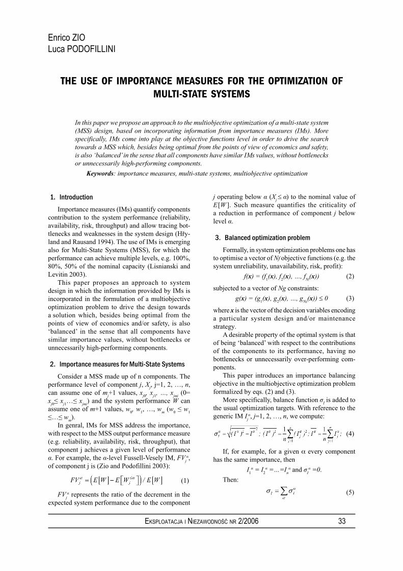
33EKSPLOATACJA I NIEZAWODNOŚĆ NR 2/2006
Enrico ZIOLuca PODOFILLINI
THE USE OF IMPORTANCE MEASURES FOR THE OPTIMIZATION OF
MULTI-STATE SYSTEMS
In this paper we propose an approach to the multiobjective optimization of a multi-state system
(MSS) design, based on incorporating information from importance measures (IMs). More
specifically, IMs come into play at the objective functions level in order to drive the search
towards a MSS which, besides being optimal from the points of view of economics and safety,
is also ‘balanced’ in the sense that all components have similar IMs values, without bottlenecks
or unnecessarily high-performing components.
Keywords: importance measures, multi-state systems, multiobjective optimization
1. Introduction
Importance measures (IMs) quantify components contribution to the system performance (reliability, availability, risk, throughput) and allow tracing bot-tlenecks and weaknesses in the system design (Hřy-land and Rausand 1994). The use of IMs is emerging also for Multi-State Systems (MSS), for which the performance can achieve multiple levels, e.g. 100%, 80%, 50% of the nominal capacity (Lisnianski and Levitin 2003).
This paper proposes an approach to system design in which the information provided by IMs is incorporated in the formulation of a multiobjective optimization problem to drive the design towards a solution which, besides being optimal from the points of view of economics and/or safety, is also ‘balanced’ in the sense that all components have similar importance values, without bottlenecks or unnecessarily high-performing components.
2. Importance measures for Multi-State Systems
Consider a MSS made up of n components. The performance level of component j, X
j, j=1, 2, …, n,
can assume one of mj+1 values, x
j0, x
j1, …, x
jmj (0=
xj0≤ x
j1…≤ x
jmj) and the system performance W can
assume one of m+1 values, w0, w
1, …, w
m (w
0 ≤ w
1
≤…≤ wm).
In genral, IMs for MSS address the importance, with respect to the MSS output performance measure (e.g. reliability, availability, risk, throughput), that component j achieves a given level of performance α. For example, the α-level Fussell-Vesely IM, FV
jα,
of component j is (Zio and Podofillini 2003):
(1)
FVjα represents the ratio of the decrement in the
expected system performance due to the component
j operating below α (Xj ≤ α) to the nominal value of
E[W ]. Such measure quantifies the criticality of a reduction in performance of component j below level α.
3. Balanced optimization problem
Formally, in system optimization problems one has to optimise a vector of Nf objective functions (e.g. the system unreliability, unavailability, risk, profit):
f(x) = (f1(x), f
2(x), …, f
Nf(x)) (2)
subjected to a vector of Ng constraints:
g(x) = (g1(x), g
2(x), …, g
Ng(x)) ≤ 0 (3)
where x is the vector of the decision variables encoding a particular system design and/or maintenance strategy.
A desirable property of the optimal system is that of being ‘balanced’ with respect to the contributions of the components to its performance, having no bottlenecks or unnecessarily over-performing com-ponents.
This paper introduces an importance balancing objective in the multiobjective optimization problem formalized by eqs. (2) and (3).
More specifically, balance function σI is added to
the usual optimization targets. With reference to the generic IM I
jα, j=1, 2, …, n, we compute:
(4)
If, for example, for a given α every component has the same importance, then
I1
α = I2
α =…=In
α and σIα =0.
Then:
(5)

34 EKSPLOATACJA I NIEZAWODNOŚĆ NR 2/2006
NAUKA I TECHNIKA
is taken as a measure of the system balance. If σIα = 0
for every α, then σI = 0 and the system is fully balanced,
free of bottlenecks or over-reliable components.
4. Application to multi-state system design
Consider a system made up of n = 3 multi-state components in series logic. Each component has m
j = 4 nonzero performance states with values of
performance xj0= 0, x
j1= 25, x
j2= 50, x
j3= 75, x
j4= 100,
j=1, 2, 3. Let pjk be the probability of component j of
being in state k. Each of the three components has to be properly selected among the 11 available choices in Table 1, respectively. The alternatives differ in their state probability distributions and costs.
The design objectives to optimize are the expected system performance E[W ] and the system balance
Table 1. Data for the eligible alternatives
Component 1 Component 2 Component 3
# p10
p12
p12
p13
p14
p20
p22
p22
p23
p24
p30
p32
p32
p33
p34
Cost
1 0.500 0.000 0.000 0.000 0.500 0.450 0.000 0.100 0.000 0.450 0.400 0.100 0.000 0.100 0.400 1.0
2 0.001 0.001 0.997 0.001 0.000 0.050 0.000 0.900 0.050 0.000 0.100 0.100 0.700 0.100 0.000 2.0
3 0.001 0.500 0.400 0.001 0.098 0.001 0.400 0.500 0.001 0.098 0.100 0.400 0.400 0.100 0.000 2.2
4 0.000 0.250 0.500 0.250 0.000 0.000 0.200 0.600 0.200 0.000 0.000 0.200 0.600 0.200 0.000 3.0
5 0.200 0.200 0.200 0.200 0.200 0.200 0.300 0.200 0.100 0.200 0.350 0.200 0.100 0.200 0.150 3.5
6 0.001 0.001 0.500 0.200 0.298 0.001 0.200 0.500 0.001 0.298 0.050 0.050 0.400 0.200 0.300 3.7
7 0.000 0.001 0.001 0.998 0.000 0.000 0.010 0.040 0.900 0.050 0.000 0.100 0.000 0.800 0.100 4.0
8 0.001 0.001 0.001 0.600 0.397 0.000 0.050 0.050 0.600 0.300 0.050 0.100 0.050 0.400 0.400 4.2
9 0.001 0.001 0.200 0.300 0.498 0.001 0.001 0.100 0.400 0.498 0.000 0.100 0.200 0.350 0.350 4.5
10 0.050 0.050 0.100 0.400 0.400 0.050 0.050 0.100 0.300 0.500 0.050 0.050 0.000 0.300 0.600 4.7
11 0.001 0.000 0.000 0.000 0.999 0.050 0.000 0.000 0.050 0.900 0.000 0.100 0.000 0.100 0.800 5.0
Table 2. Non-dominated designs (problem 1).
Design
#E[W] σ
ICost j = 1 j = 2 j = 3
1 84.420 0.616 15.0 11 11 11
2 78.730 0.535 14.7 11 11 10
3 71.460 0.424 13.7 8 9 11
4 69.220 0.315 13.4 8 9 10
5 68.580 0.137 12.0 7 7 7
6 66.560 0.106 12.2 7 8 7
7 63.840 0.103 12.5 7 7 9
8 62.070 0.086 12.7 7 8 9
9 56.930 0.079 12.7 9 9 6
10 52.820 0.075 11.9 6 9 6
11 46.120 0.071 10.2 2 9 6
12 45.860 0.052 11.5 4 7 9
13 44.170 0.029 11.0 9 9 2
14 42.380 0.028 8.5 2 9 2
15 41.040 0.024 10.0 4 7 4
16 37.250 0.009 9.0 4 4 4
Table 3. Non-dominated designs (problem 2).
Design #
E[W] σI
Cost j = 1 j = 2 j = 3
1 49.520 0.090 11.0 7 7 4
2 46.120 0.071 10.2 2 9 6
3 44.170 0.029 11.0 9 9 2
4 42.380 0.028 8.5 2 9 2
5 41.040 0.024 10.0 4 7 4
6 37.250 0.009 9.0 4 4 4
σFV
with respect to the generalized Fussell-Vesely IM, FV
jα of eq. (1).In optimisation problem 1, we do not consider
constraints on the total allocation cost, whereas the case of a maximum allocation cost C
max is considered
in optimisation problem 2. The search space (11·11·11 alternative designs) has been spanned in both cases. The non-dominated solutions are listed in decreasing order of E[W ] in Table 2 and Table 3 for optimisation problems 1 and 2, respectively.
For problem 1, we report in Figure 1 the values of FV
j≤α (left) α = 0, 25, 50, 75, j = 1, 2, 3, and p
jk (right),
k = 0, 1, …, 4, j = 1, 2, 3, for solution 1 of Table 2, the best with respect to the expected performance E[W ], and in Figure 1. the values for solution 16, the best with respect to σ
FV.
The best solution with respect to E[W] (solution 1 in Table 2) corresponds to the design vector x1 = (11; 11; 11), where alternative 11 is the most performing for all three components, i.e. the one with state probability distribution most shifted towards high-performance states. Figure 1 (left) shows the values of FV
j≤α, j = 1,
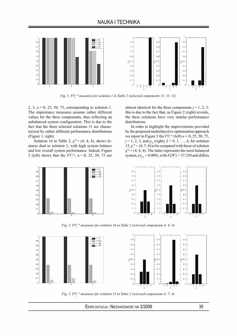
35EKSPLOATACJA I NIEZAWODNOŚĆ NR 2/2006
NAUKA I TECHNIKA
Fig. 1. FVj<α measures for solution 1 in Table 2 (selected components 11; 11; 11)
Fig. 2. FVj<α measures for solution 16 in Table 2 (selected components 4; 4; 4)
Fig. 3. FVj<α measures for solution 15 in Table 2 (selected components 4; 7; 4)
2, 3, α = 0, 25, 50, 75, corresponding to solution 1. The importance measures assume rather different values for the three components, thus reflecting an unbalanced system configuration. This is due to the fact that the three selected solutions 11 are charac-terized by rather different performance distributions (Figure 1, right).
Solution 16 in Table 2, x16 = (4; 4; 4), shows fe-atures dual to solution 1, with high system balance and low overall system performance. Indeed, Figure 2 (left) shows that the FV
j≤α, α = 0, 25, 50, 75 are
almost identical for the three components j = 1, 2, 3: this is due to the fact that, as Figure 2 (right) reveals, the three solutions have very similar performance distributions.
In order to highlight the improvements provided by the proposed multiobjective optimisation approach we report in Figure 3 the FV
j≤α (left) α = 0, 25, 50, 75,
j = 1, 2, 3, and pjk (right), k = 0, 1, …, 4, for solution
15, x15 = (4; 7; 4) to be compared with those of solution x16 = (4; 4; 4). The latter represents the most balanced system, (σ
FV = 0.009), with E[W ] = 37.250 and differs
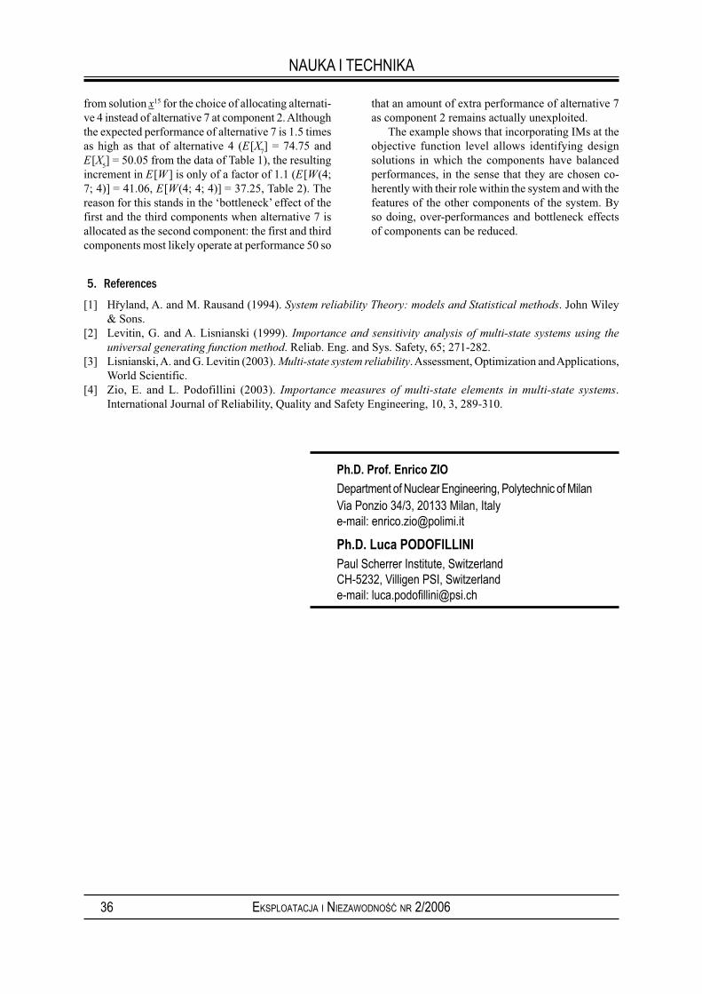
36 EKSPLOATACJA I NIEZAWODNOŚĆ NR 2/2006
NAUKA I TECHNIKA
from solution x15 for the choice of allocating alternati-ve 4 instead of alternative 7 at component 2. Although the expected performance of alternative 7 is 1.5 times as high as that of alternative 4 (E[X
7] = 74.75 and
E[X5] = 50.05 from the data of Table 1), the resulting
increment in E[W ] is only of a factor of 1.1 (E[W(4; 7; 4)] = 41.06, E[W(4; 4; 4)] = 37.25, Table 2). The reason for this stands in the ‘bottleneck’ effect of the first and the third components when alternative 7 is allocated as the second component: the first and third components most likely operate at performance 50 so
that an amount of extra performance of alternative 7 as component 2 remains actually unexploited.
The example shows that incorporating IMs at the objective function level allows identifying design solutions in which the components have balanced performances, in the sense that they are chosen co-herently with their role within the system and with the features of the other components of the system. By so doing, over-performances and bottleneck effects of components can be reduced.
5. References
[1] Hřyland, A. and M. Rausand (1994). System reliability Theory: models and Statistical methods. John Wiley & Sons.
[2] Levitin, G. and A. Lisnianski (1999). Importance and sensitivity analysis of multi-state systems using the
universal generating function method. Reliab. Eng. and Sys. Safety, 65; 271-282.[3] Lisnianski, A. and G. Levitin (2003). Multi-state system reliability. Assessment, Optimization and Applications,
World Scientific.[4] Zio, E. and L. Podofillini (2003). Importance measures of multi-state elements in multi-state systems.
International Journal of Reliability, Quality and Safety Engineering, 10, 3, 289-310.
Ph.D. Prof. Enrico ZIO
Department of Nuclear Engineering, Polytechnic of MilanVia Ponzio 34/3, 20133 Milan, Italye-mail: [email protected]
Ph.D. Luca PODOFILLINIPaul Scherrer Institute, SwitzerlandCH-5232, Villigen PSI, Switzerlande-mail: luca.podofi [email protected]

37EKSPLOATACJA I NIEZAWODNOŚĆ NR 2/2006
Ilia FRENKELLev KHVATSKIN
COST – EFFECTIVE MAINTENANCE WITH PREVENTIVE REPLACEMENT OF
OLDEST COMPONENTS
We consider preventive maintenance of a continuously operating system, whose real-life pro-
totype is a rotating chemical reactor for production of phosphorous acid. The drum, in which
the reaction takes place, has 42 rollers (elements), which are subjected to a heavy load and to
chemical corrosion. The components are organized in a ring-type structure. The system failure
is defined either as the failure of 2 adjacent elements, or as a failure of any three elements in
a set of 6 adjacent elements. The existing servicing policy prescribes replacing only the failed
elements at the instant of system failure occurrence. The operational conditions permit the
opportunistic replacement of non-failed components at the instant of system failure.
In this paper, we propose a cost-effective policy of preventive maintenance: at the same time
the system fails, several of the oldest non-failed components are replaced by new ones. The
application of the above optimal preventive maintenance policy results in a reduction of the
average cost per unit time by 15-30%.
Keywords: preventive maintenance, group replacement, simulation approach
1. Introduction
Group replacement is one of the strategies that may be employed for the maintenance of technical systems of identical, consecutive components. The aim of the strategy is to replace all or part of the system’s com-ponents within given time periods, thus minimizing the maintenance costs (Gertsbakh 2000).
It is possible to plan the repair, either on the basis of operational time elapsed since the last repair or when a critical number of elements failed to function. It is natural to replace preventively the oldest elements among the non-failed ones. In order to ensure opti-mum efficiency in the latter maintenance approach, we introduce two parameters: a threshold of failures, necessary for implementing the repair; and the number of components to be replaced (Dekker et al. 2000).
It is extremely difficult to investigate a problem of this type analytically. Consequently, we propose an ap-proach and a solution based on a simulation study.
2. Problem Description
We consider a system consisting of n independent statistically identical components. It is assumed that 2 adjacent malfunctioning components cause the sys-tem to come to a halt. At the instant the system stops, the components that have failed are replaced by new identical ones. We assume that the replacement time is negligible. The cost of the replacement is constant and is C
1, while the cost of the breakdown of the sys-
tem is C0. Thus a repair involving the replacement of
the malfunctioning component, as well as the r oldest elements, will cost the following sum: C
0+(r+2)C
1.
The renewal of the broken elements with the simultaneous replacement of r oldest elements leads both to a decrease in the number of breakdowns when the system is in use, and conversely to an increase in the periods between repairs. The aim of this study is to establish the optimal r, which minimizes the main-tenance cost per unit time.
The expected cost of maintenance per time unit is stated as a function of the number of r components and is given by the following formula (Frenkel et al. 2002):
(1)
where E[N ] represents the mean value of failures occurred in the [0,T] interval.
The simulation algorithm is written in MA-TLAB.
3. Case Study
The real-life prototype for n-component system is the Phosphor acid filter, using in Rotem/Deshanim Chemical Processing Facility, Arad, Israel, whose base is comprised of 42 identical turning rollers (elements). According to the technical specification, a failure (bre-akdown) of the system occurs when 2 adjacent rollers stop working. The cost of the system’s breakdown is $100. The cost of replacing an element varies from $1 to $99. Time to failure for one roller, according to
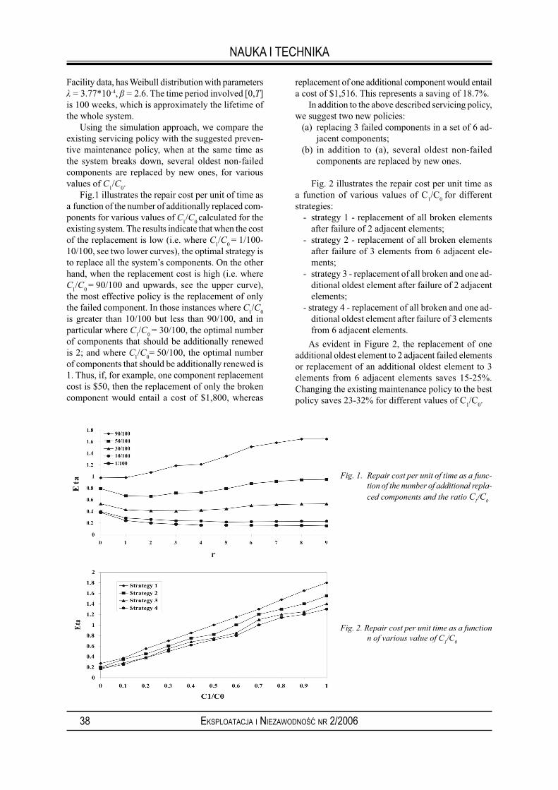
38 EKSPLOATACJA I NIEZAWODNOŚĆ NR 2/2006
NAUKA I TECHNIKA
Facility data, has Weibull distribution with parameters λ = 3.77*10-4, β = 2.6. The time period involved [0,T] is 100 weeks, which is approximately the lifetime of the whole system.
Using the simulation approach, we compare the existing servicing policy with the suggested preven-tive maintenance policy, when at the same time as the system breaks down, several oldest non-failed components are replaced by new ones, for various values of C
1/C
0.
Fig.1 illustrates the repair cost per unit of time as a function of the number of additionally replaced com-ponents for various values of C
1/C
0 calculated for the
existing system. The results indicate that when the cost of the replacement is low (i.e. where C
1/C
0 = 1/100-
10/100, see two lower curves), the optimal strategy is to replace all the system’s components. On the other hand, when the replacement cost is high (i.e. where C
1/C
0 = 90/100 and upwards, see the upper curve),
the most effective policy is the replacement of only the failed component. In those instances where C
1/C
0
is greater than 10/100 but less than 90/100, and in particular where C
1/C
0 = 30/100, the optimal number
of components that should be additionally renewed is 2; and where C
1/C
0= 50/100, the optimal number
of components that should be additionally renewed is 1. Thus, if, for example, one component replacement cost is $50, then the replacement of only the broken component would entail a cost of $1,800, whereas
replacement of one additional component would entail a cost of $1,516. This represents a saving of 18.7%.
In addition to the above described servicing policy, we suggest two new policies:
(a) replacing 3 failed components in a set of 6 ad-jacent components;
(b) in addition to (a), several oldest non-failed components are replaced by new ones.
Fig. 2 illustrates the repair cost per unit time as a function of various values of C
1/C
0 for different
strategies:- strategy 1 - replacement of all broken elements
after failure of 2 adjacent elements;- strategy 2 - replacement of all broken elements
after failure of 3 elements from 6 adjacent ele-ments;
- strategy 3 - replacement of all broken and one ad-ditional oldest element after failure of 2 adjacent elements;
- strategy 4 - replacement of all broken and one ad-ditional oldest element after failure of 3 elements from 6 adjacent elements.
As evident in Figure 2, the replacement of one additional oldest element to 2 adjacent failed elements or replacement of an additional oldest element to 3 elements from 6 adjacent elements saves 15-25%. Changing the existing maintenance policy to the best policy saves 23-32% for different values of C
1/C
0.
Fig. 1. Repair cost per unit of time as a func-
tion of the number of additional repla-
ced components and the ratio C1/C
0
Fig. 2. Repair cost per unit time as a function
n of various value of C1/C
0

39EKSPLOATACJA I NIEZAWODNOŚĆ NR 2/2006
NAUKA I TECHNIKA
4. Conclusion
In summation, it is proposed that an optimal policy of maintenance, for a system consisting of identical and independent components, be based on the replacement of both the failed components and a certain number of the oldest but still functioning components.
It has been demonstrated that this strategy of gro-up replacement compares very favorably with that of simply replacing the failed components and that it guarantees savings in the range of 15-32%.
5. References
[1] Gertsbakh, I.B. (2000): Reliability Theory with Applications to Preventive Maintenance, Berlin: Springer-Verlag.
[2] Dekker R. et al. (1998): Maintenance of light-standards: a Case Study. Journal of the Operational Research Society, 49: 132-143.
[3] Frenkel, I.B., Khvatskin, L.V. and Laslo, Z. (2002): A Preventive Maintenance Policy: Simultaneous Replacement
of the Oldest Components in Addition to the Failed Component. Communications in Dependability and Quality
Management, An International Journal, 5(2), p. 89-96.
Ph.D. Ilia FRENKELPh.D. Lev KHVATSKIN
International Reliability and Risk Management Center Sami Shamoon College of Engineering Beer Sheva, 84100, Israel e-mail: [email protected] / [email protected]

40 EKSPLOATACJA I NIEZAWODNOŚĆ NR 2/2006
Alexander ROTSHTEINSerhiy SHTOVBA
MODELING OF ALGORITHMIC PROCESS RELIABILITY WITH FUZZY
SOURCE DATA
This paper proposes the method, which allows predicting such reliability figures of a discrete
algorithmic process as the fuzzy time and the fuzzy probability of correct execution. Fuzzy
numbers represents the uncertain source modeling data. Fuzzy rule bases used for taking into
account dependence of source data on many influencing factors. Fuzzy logic inference, fuzzy
extension principle together the crisp reliability models of algorithmic processes are used for
modeling.
Keywords: Fuzzy Reliability, Algorithmic Process, Fuzzy Number, Fuzzy Extension
Principle
1. Introduction
Many discrete-behavior systems can be analyzed in a unified framework if combined into a class of so-called algorithmic processes. Typical algorithmic processes include information processing in computer systems, performance of research or design projects, technological production processes etc. Each of these processes involves a sequence of operations or jobs unfolding in time whose execution leads to the goal achievement. When designing a specific algorithmic process (AP), we need to estimate of the following reliability figures: � p
AP – the probability of correct AP execution;
this may be interpreted as the reliability of out-put information, defect-free quality of the output products, reliability of system functioning;
� tAP
– the time or other resources required to exe-cute the AP.
Models to estimate pAP
and tAP
are widely used in reliability theory of man-machine systems [1, 2, 3]. In these studies, the modeling is based on the theory of semi-Markov processes [4] whose states correspond to the operators and logical conditions of the given algorithm. Successful application of AP reliability theory envisages construction of databases with reliability characteristics of the basic elementary operations. However, new operations do not have ex-post statistical estimates of outcomes under real-life conditions. Complex-system designers are therefore often forced to make decisions on the basis of fol-lowing expert judgments: “if the human operator
is tired, then the number of errors is approximately
doubled” or “if the equipment is properly maintained
and is operated under appropriate conditions, then
the reliability is high”.
The probabilistic algorithmic reliability theory [1, 2, 3] is incapable of utilizing input data expressed in the form of natural-language expert judgments. It is therefore relevant to try and develop a so-called “fuzzy reliability theory of algorithmic processes” [5, 6, 7], which together the probabilistic approach also uses fuzzy set theory [8], [9] that can manipulate linguistic expert information.
In this article we propose an approach that extends the probabilistic AP’s reliability models to the case of fuzzy input data and allows for the dependence of data on influential factors through fuzzy inference. In terms of fuzzy reliability [10], extended AP’s relia-bility models one can account as a branch of probist reliability theory with fuzzy probabilities.
2. Language for description the algorithmic processes
For formal description of AP we use the language of Glushkov’s algorithmic algebras [11]. In this lan-guage, the algorithm operators are denoted by Latin capital letters (A, B, C, …) and logical conditions are denoted Greek lower-case letters (α, β, γ, …). By the regularization theorem [11], every algorithm is re-presentable a superposition of the following operator structures: � B=A
1A
2 – linear structure consists of the process
of consecutive operators A1 and A
2 execution in
the order of their registration;
� – α-disjunction representing ope-rator A
1 execution when condition α is true (α=1),
and execution of operator A2 when condition α is
α=0);
� – α-iteration representing cyclic exe-cution of operator A till condition α has become true.
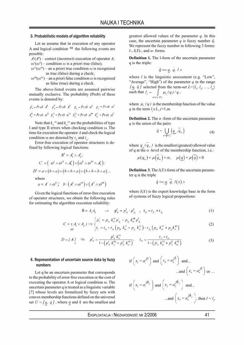
41EKSPLOATACJA I NIEZAWODNOŚĆ NR 2/2006
NAUKA I TECHNIKA
greatest allowed values of the parameter q. In this case, the uncertain parameter q is fuzzy number . We represent the fuzzy number in following 3 forms: l-, l(X)-, and α- forms.
Definition 1. The l-form of the uncertain parameter q is the triple:
where l is the linguistic assessment (e.g. “Low”, “Average”, “High”) of the parameter q in the range
selected from the term-set L={l1, l
2, …, l
m}
such that ,
where is the membership function of the value q in the term l
j∈L, j=1,m.
Definition 2. The α -form of the uncertain parameter q is the union of the pairs
(4)
where is the smallest (greatest) allowed value of q at the α -level of the membership function, i.e.:
Definition 3. The l(X )-form of the uncertain parame-ter q is the triple
where l(X ) is the expert knowledge base in the form of systems of fuzzy logical propositions:
3. Probabilistic models of algorithm reliability
Let us assume that in execution of any operator A and logical condition the following events are possible:A1(A0) – correct (incorrect) execution of operator A; ω1(ω0) – condition ω is a priori true (false); ω11(ω10) – an a priori true condition ω is recognized
as true (false) during a check; ω00(ω01) – an a priori false condition ω is recognized
as false (true) during a check.
The above-listed events are assumed pairwise mutually exclusive. The probability (Prob) of these events is denoted by:
Note that kω
10 and kω
01 are the probabilities of type I and type II errors when checking condition ω. The time for execution the operator A and check the logical condition ω are denoted by t
A and t
ω.
Error-free execution of operator structures is de-fined by following logical functions:
where
Given the logical functions of error-free execution of operator structures, we obtain the following rules for estimating the algorithm execution reliability:
(1)
(2)
(3)
4. Representation of uncertain source data by fuzzy
numbers
Let q be an uncertain parameter that corresponds to the probability of error-free execution or the cost of executing the operator A or logical condition ω. The uncertain parameter q is treated as a linguistic variable [7] whose levels are formalized by fuzzy sets with convex membership functions defined on the universal set , where and are the smallest and
if and and...
...and or …
if and and...
...and , then l = lj,
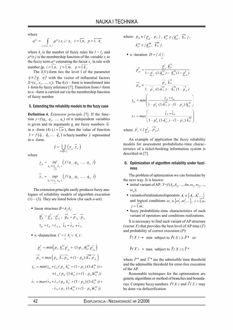
42 EKSPLOATACJA I NIEZAWODNOŚĆ NR 2/2006
NAUKA I TECHNIKA
where
where kj is the number of fuzzy rules for l = l
j, and
μip(xi) is the membership function of the variable x
i to
the fuzzy term aijp estimating the factor x
i in rule with
number jp, The l(X( )-form ties the level l of the parameter
with the vector of influential factors X=(x
1, x
2, …, x
n). The l(x) – form is transformed into
l–form by fuzzy inference [7]. Transition from l–form to α –form is carried out via the membership function of fuzzy number.
5. Extending the reliability models to the fuzzy case
Definition 4. Extension principle [7]. If the func-tion y =f (q
1, q
2, …, q
n) of n independent variables
is given and its arguments qi are fuzzy numbers
in α -form (4) ( ), then the value of function is fuzzy number represented
in α -form:
where
The extension principle easily produces fuzzy ana-logues of reliability models of algorithm execution (1) – (3). They are listed below (for each α-set):
� linear structure B=A1A
2:
,
,
� α -disjunction :
where: , ,
.
� α -iteration :
where .
An example of application the fuzzy reliability models for assessment probabilistic-time charac-teristics of a ticket-booking information system is described in [7].
6. Optimization of algorithm reliability under fuzzi-
ness
The problem of optimization we can formulate by the next way. It is known:� initial variant of AP: Y=f (A
1,A
2, ..., An, ω
1, ω
2, ...,
ωm);
� variants of realization of operators and logical conditions , ,
;� fuzzy probabilistic-time characteristics of each
variant of operators and conditions realizations.
It is necessary to find such variant of AP structure (vector X ) that provides the best level of AP time (T) and probability of correct execution (P):
min subject to or
max subject to
where and are the admissible time threshold and the admissible threshold for error-free execution of the AP.
Reasonable techniques for the optimization are genetic algorithms or method of branches and bounda-
ries. Compare fuzzy numbers and may be done via defuzzification.

43EKSPLOATACJA I NIEZAWODNOŚĆ NR 2/2006
NAUKA I TECHNIKA
6. Conclusions
The main obstacle to the application of probabili-stic reliability models is the absence of input data that reflect real-life conditions describing the operation of the system. The method proposed in this paper for esti-mating the reliability of algorithms is one of the formal approaches to resolving the difficulty with source data
by means of linguistic expert information and fuzzy extension principle. Contrary to semi-Markov models used in reliability theory, the proposed technique is free from time-consumed procedures for convolution of the distribution functions of the system sojourn time in a given state.
7. References
[1] Gubinskii, A.I. (1982): Reliability and Operating Quality of Ergatic Systems. Leningrad: Nauka. [In Russian].
[2] Rotshtein, A. (1990): Algebraic Design of Fault-Free Labour Processes. Upr. Sist. Mash., No. 6, P. 92-102. [3] Rotshtein A.: Probabilistic-Algorithmic Models of Man-Machine Systems // Soviet Journal Automation and
Information Science.– 1987, No 5. P.81-86. [4] Korolyuk, V.S. and Turbin, A.F. (1976): Phase Aggregation of Complex Systems, Kiev: Vishcha Shkola. [In
Russian]. [5] Rotshtein, A. (1994): Fuzzy reliability analysis of man-machine systems. In Reliability and Safety Analysis
under Fuzziness, Studies in Fuzziness, Berlin: Physika-Verlag, Springer-Verlag, pp. 245-270. [6] Rotshtein, A. and Shtovba, S. (1997): Fuzzy Reliability Analysis and Optimization of Algorithmic Processes
// Proc. of the Fifth European Congress on Intelligent Techniques and Soft Computing, Germany, Aachen, pp. 67-71.
[7] Rotshtein, A. and Shtovba, S. (1998): Prediction the Reliability of Algorithmic Processes with Fuzzy Input
Data. Cybernetics and Systems Analysis. Vol. 34., No.4, pp.545-552. [8] Zadeh, L. (1965): Fuzzy Sets // Information and Control. Vol.8, pp.338-358. [9] Zimmerman, H.-J. (1996): Fuzzy Set Theory and its Applications. Kluwer Academic Publishers, Dordrecht.[10] Cai, K.-Y. (1996): Introduction to Fuzzy Reliability. Kluwer Academic Publishers, Dordrecht.[11] Glushkov, V. M., Tseitlin, G. E., and Yushchenko, E. L. (1978): Algebra. Languages. Programming. Kiev:
Naukova Dumka. [In Russian].
Ph.D. Alexander ROTSHTEIN
Industrial Engineering and Management Department Jerusalem College of Technology – Machon Lev21 HaVaad HaLeumi St., Givat Mordechai, Jerusalem, 91160, Israele-mail: [email protected]
Ph.D. Serhiy SHTOVBA
Computer Based Information and Management Systems DepartmentVinnitsa National Technical UniversityKhmelnitskoe Shosse, 95, Vinnitsa, 21021, Ukrainee-mail: [email protected]

44 EKSPLOATACJA I NIEZAWODNOŚĆ NR 2/2006
Boyan DIMITROVDavid GREENVladimir RYKOVPeter STANCHEV
ON THE FAIR SHARE OF THE RELIABILITY OF AN ENTITY
BETWEEN ITS COMPONENTS
The problem of the reliability of an entity sharing between their components in order to maximize
its lifetime is considered. Some algorithms generating solutions to the problem is presented
along with numerical examples for the problem.
Keywords: optimization, reliability systems, lifetime maximization
1. Introduction
Most of real engineering entities (products, go-ods) consists of various components and usually has a complex hierarchical structure. Their components have different reliability, cost and other characteristics. The entity’s reliability is usually determined by the reliability of the weakest component among them. Thus, it then becomes necessity to investigate how to construct the system in order to uniformly maximize its reliability. As mathematical tools for investigation of these kinds of systems the multi-state system relia-bility models could be used.
The problem of multi-state system reliability investigation was considered by different authors, and one can find the bibliography in Lisnianski and Levitin (2003). Some special approach to this problem for complex hierarchical systems also was developed in several papers (Dimitrov et al. 2004, Dimitrov et al. 2002, Dimitrov and Rykov 2002). Some problems of reliability control were considered in Rykov and Efrosinin (2004). In (Ermolaev and Rykov 2000) the problem of optimal reservation with different types of equipment was considered. In this paper we consider the problem of a system reliability sharing between its components with respect to the system lifetime maximization.
2. Problems settings
Consider an entity consisting of m components having lifetimes T
i with cumulative probability
distribution functions (c.d.f.) Fi(t) (i = 1,2,...,m).
Denote by Ri(t) = 1-F
i(t) the reliability functions of
the i–th component. Suppose that in accordance with consumer requirements the entity should be given reliability function of level at least r = 1-α. It means that the probability for the entity to fail should be only α, or less.
The usual opinion that the equally reliable com-ponents provide the best reliability for the system is not really true. To explain this fact let us consider the following examples.
2.1. Consequence system
For a system with consequently connected com-ponents, each of which has an exponential lifetime di-
stribution with parameters λi i m, = , ,( )1 the reliability function of the system equals (Gertsbakh 2000)
R t t ei m
i
t( ) exp= −⎧⎨⎩
⎫⎬⎭
≡≤ ≤
⎛
⎝
⎜⎜⎜
⎞
⎠
⎟⎟⎟
−∑1
λ Λ with Λ =≤ ≤∑
1 i m
iλ
The reliability level r = 1-α will be provided up to time t1
1−
−= − ≈α
α αln( )Λ Λ
. The reliability level of i-th component of the system for this time will be equal
R t ei
t ii
ii
( ) exp ln( ) ( )11 1 1 1−
−= = −⎧⎨⎩
⎫⎬⎭
= − = − .−α
λ α
λλα α α
ΛΛ
Note that the equally reliable sharing of the pro-bability between subsystems when reliability level for each component equals (1-α)1/m provides the guaran-teed lifetime for i-th component only
tm m
i
i i
, − = − − ≈ .1
11α
λα
α
λln( )
Thus, the (1-α) guaranteed lifetime level for a sys-tem will be equal
t tm mi m
i
i i
1 1 1
1 1− ≤ ≤ , −= = −
−≈α α
α
λ
α
λmin
ln( )
max max
If we consider some simple case of the system with only two components with parameters λ
1 = 0.1
and λ2 = 0.01 then the equally reliable sharing of the
system reliability provides 1-α guaranteed lifetime equals t
1-α= min[5α,50α] = 5α, while an optimal sha-

45EKSPLOATACJA I NIEZAWODNOŚĆ NR 2/2006
NAUKA I TECHNIKA
ring provide the time t1 9 09−∗ =≈ .α α , that gives almost
twice longer time.
2.2. Parallel system
For a system with parallel connected components, each of which has an exponential lifetime distribution
with parameters λi i m, = , ,( )1 the reliability function of the system equals (Gertsbakh 2000)
R t ei m
ti( ) ( )= − − .≤ ≤
−∏1 11
λ
Thus, for any given reliability level of the system r = 1-α in order to reach the guaranteed lifetime t
1-α
of the system one should provide the reliability level
of i-th component equal R t ei
ti( ) )1
1−
−= −α
λ α . For enough reliable systems with reliability level of components
close to one, this gives r e ti i
t
ii= − = ≈ −−
−−1 11
1α λλ
αα ) ,
or αi ≈ λ
it1-α
. This shows that the level of i-th compo-nent to fail should be proportional to the failure inten-sity. One could find the proportionally coefficient c from the equality α α λ= = .
≤ ≤ ≤ ≤∏ ∏1 1i m i
m
i m ic From this equality it follows that
c
m
i m i
=⎛
⎝⎜⎜
⎞
⎠⎟⎟
,≤ ≤∏
1
1
α
λ
and thus
α λα
λi i
i m i
m
=⎛
⎝⎜⎜
⎞
⎠⎟⎟
.≤ ≤∏
1
1
This shows the difference between reliability levels of the components.
These examples show that the reliability level for different components of the system should be diffe-rent in order to provide maximal guaranteed lifetime of the system. Thus the problem arise how to share of given level of the reliability of a system between its components.
In mathematical terms the problem could be formu-lated as follows. Suppose that the entity consists of m
components with reliability functions R t i mi ( ) ( )= ,1, and has a structure function f(x)=f(x
1,x
2,...,x
m). This
means that the reliability function of the entity is (see, Gertsbakh 2000).
R t f x x & x f R t R t &R tm m( ) [ ( )] ( ( ) ( ) ( ))= , , , = , ,E 1 2 1 2 (1)
Thus, one should choose a point r = , ,( )r r & rm1 2 in the hyper-space
f(r1,r
2,...,r
m)≥r=1-α with
d r r & r r i mm i{( ) ( )}1 2 0 1 1, , : ≤ ≤ = , (2)
in such a way to maximize
t R11 1−
−= − ⇒α α( ) max (3)
3. Problems solution
A theoretical solution of the problem is very simple. If one know the reliability function of the system (1) he/she can solve (at least in principle) an equation
R(t) = r =1-α (4)
to find t1-α
= R-1(1-α). Due to usual strong monotonicity of the function R(t) the solution exists and unique. Thus, the reliability level of each component equals r
i = 1-α
i = R
i(t
1-α).
Nevertheless, because the reliability function R(t) in real world problems is enough complicated and moreover it is composition of several functions: structure function of a system and reliability functions of its components – the exact solution of this equation is really impossible.
Because any monotone system can be represented as a system of consequence-parallel structure we will consider here these types of structures. We propose euristical algorithms for the problem solution for two cases: consequence and parallel systems.
To reliability share for consequence system it is possible to use the following algorithm
3.1. Algorithm 1. Series system
Input initial data: Integer: m – number of subsystems; Real: ε – accuracy coefficient, r – consumer’s relia-bility level; Functions: R
i(t) – reliability functions.
Begin. Find an initial point r( ) ( ) ( )( )0
10 0= , ,r & rm at the
hyper-space
f r r r r & r r i mi m
i m i( ) {( ) ( )}r = = , , , : ≤ ≤ = ,≤ ≤∏
11 2 0 1 1 (5)
For series system as an initial point it is possible to take r
i(0) = r1/m. Go to the step 1 with k = 0.
Step 1. For inverse functions Ri(-1)(·) calculate
ti(k) = R
i(1)(r
i(k)) and arrange them in order to increasing
t t & ti
k
i
k
i
k
m1 2
( ) ( ) ( )≤ ≤ ≤ ,
where ij denotes the number of component having j-th
in order lifetime. Step 2. Check if t ti
k
i
k
m
( ) ( )− ≤1
ε go to the step 4, in other case go to the step 3. Step 3. Change the point r at the hyper-space (5) in or-der to decrease ri1
and increase rim. For example, with
some improvement coefficient γ < 1 put r ri
k
i
k
1 1
1+ = γ and r ri
k
i
k
m m
+ −=1 1γ . Change k to k+1. Go to the step 1 with new value of r
ik+1.

46 EKSPLOATACJA I NIEZAWODNOŚĆ NR 2/2006
NAUKA I TECHNIKA
Step 4.Print results. End
For the systems with parallel connection one sho-uld work with fail probabilities instead of subsystems reliability. Thus the algorithm looks like this one.
3.2. Algorithm 2. Parallel system
Input initial data: Integer: m – number of subsystems; Real: ε – accuracy coefficient, α – probability level for the entity to fail; Functions: F
i(t) – lifetimes c.d.f.
Begin. Find an initial point (α1(0),..., α
m(0)) with α
i(0) = 1-
ri(0) at the hyper-space
1
1
− = = ,≤ ≤∏f
i m
i( )r α α
{( ) ( )}α α α1 0 1 1, , : ≤ ≤ = , .& i mm i (6)
For parallel system as an initial point it is possible to take α
i(0) = α1/m. Go to the step 1 with k = 0.
Step 1. For inverse functions Fi(-1)(·) calculate
ti(k) = F
i(-1)(α
i(k)) and arrange them in order to incre-
asing
t t & ti
k
i
k
i
k
m1 2
( ) ( ) ( )≤ ≤ ≤
where ij denotes the number of component having j-th
in order lifetime. Step 2. Check if t ti
k
i
k
m
( ) ( )− ≤1
ε go to the step 4, in other case go to the step 3. Step 3. Change the point (α
1(k),..., α
m(k)) at the hyper-
space α α=≤ ≤∏1 i m i
in order to increase αi1 and
decrease αim. For example, with some improvement
coefficient γ > 1 put α γαi
k
i
k
1 1
1+ = and α γ αi
k
i
k
m m
+ −=1 1 . Change k to k +1. Put 1-α
ik = r
ik+1. Go to the step 1
with new values of αik+1.
Step 4. Print results. End
The results of the algorithms could be formula-ted as follows: to increase the lifetime of a system
with sequential connection of subsystem one should
strengthen the weakest component, while for the sys-
tem with parallel connection one should strengthen
the strongest one. In real world problems the exact reliability func-
tions are usually not known. A problem arise on how to use observed data instead of exact information about reliability functions. We propose a statistical approach for solving the above problem.
4. Statistical approach
In practice producers really do not have complete information about the true reliability functions of the components in use. In reality, only some statistical observations about the component’s lifetimes are
available. Thus, we also propose an approach to the solution of the problem when some statistical or mixed data are available.
Let t t & t i mi i i ni, , ,, , , = ,1 2 1( ) be the observations on the component’s lifetimes ordered in increasing their values separately for each of the components. It is well known that the best estimation for the α-percentile of a distribution is the empirical (sample) percentile, given by the formula t t
i i ii nα α= , +[ ] 1 . Thus, in the above proposed procedure one could use empirical percenti-les instead of the theoretical ones when the true lifeti-me distributions are not available. For this case only the problem arise with the stopping procedure.
Also both cases with consequence and parallel connection should be considered separately. We pro-pose an Algorithm only for consequence connection of a system.
4.1. Algorithm 3. Statistical
Input initial data: Integer: m — number of subsystems, Real: r — consumer’s reliability level; Observations: t t & t i mi i i ni, , ,, , , = ,1 2 1( ) – lifetime of components observations. Begin. Arrange the observed data in order of incre-asing values for any component
t t & t & t i mi i i l i ni i, , , ,≤ ≤ ≤ ≤ ≤ = ,1 2 1( )
Put ti(0) = t
i,1, l
i(0) = 0 ( )i m= ,1 , r
i(0)=1. Go to step 1
with k = 0. Step 1. Find t(k) = min
1≤i≤mti(k), i(k) = argmin
1≤i≤mti(k).
Step 2. Check if li(k) ≤ n
i and r(k) ≥ r go to step 3 other-
wise go to step 4. Step 3.Change k to k +1. Put l
i(k+1) = l
i(k)+1 for i = ik,
t ti
k
i lik
( )( )
+
,= +
11 for i = ik. Calculate
rn l
nr
n l
k
i m
i i
k
i
k
i i
k
( )( )
( )( )
+
≤ ≤
=−
= −−
⎛
⎝⎜
⎞
⎠⎟∏1
1
11
Go to the step 1. Step 4. Print results. End
5. Conclusion
The proposed approach considers an optimization aspect in reliability systems. It could be realized as a special Computer oriented Project and realized in different branches of industry.
Acknowledgements
One of the authors thanks the Russian Found of Fundamental Investigations for the support of the study due to the Grant Number 04-07-901156.
47EKSPLOATACJA I NIEZAWODNOŚĆ NR 2/2006
NAUKA I TECHNIKA
References
[1] Lisnianski, A. and G.Levitin (2003): Multi-State System Reliability. World Scientific. [2] Dimitrov, B., D.Green, V.Rykov and P.Stanchev (2004): Reliability of Complex Hierarchical Fault Tolerance
Systems. In Abstracts of The 4-th International Conference on Mathematical Methods in Reliability (MMR-2004), Santa Fe, (USA), 21-25 July, 2004.
[3] Dimitrov, B., D.Green, V.Rykov and P.Stanchev (2004): Reliability Model for Biological Objects. In Proceedings of The 1-st International Conference on Longevity, Aging and Degradation in Reliability, Medicine and Biology (LAD-2004), Saint Petersburg, (Russia), 7-9 July, 2004
[4] Dimitrov, B., V. Rykov(2002): On multi-state reliability systems. In Applied Stochastic Models and Information Processes. Proceedings of International Seminar. Karelian Research Center of the Russian Academy of Science. Institute of Applied Mathematical Research. Petrozavodsk, 2002. P.128-135.
[5] Dimitrov, B., V.Rykov and P.Stanchev (2002): On multi-state reliability systems. In Proceedings of the MMR 2002, Trondheim, Norway 2002. P.136-140
[6] Rykov, V., D. Efrosinin (2004): Reliability Control of Fault Tolerance Units. In: Abstracts of The 4-th International Conference on Mathematical Methods in Reliability (MMR-2004), Santa Fe, (USA), 21-25 July, 2004
[7] Ermolaev, A.I. and V.V. Rykov (2000): The problem of optimal reservation with different types of equipment.
In Second International Conference on Mathematical Methods in Reliability (MMR’2000). University Victor Segalen Bordeaux 2, Vol. 1, pp. 381-385.
[8] Gertsbakh, I. (2000): Reliability Theory with Application to Preventive Maintenance. Berlin:Springer.
Ph.D. Prof. Boyan DIMITROV Ph.D. Prof. David GREEN Ph.D. Prof. Peter STANCHEVKettering University Flint, Michigan, USAe-mail: [email protected]: [email protected]: [email protected]
Ph.D Prof. Vladimir RYKOV Russian State Oil and Gas University, Moscow, Russiae-mail: [email protected]

48 EKSPLOATACJA I NIEZAWODNOŚĆ NR 2/2006
Léo GERVILLE-RÉACHE Mikhail NIKULIN
ON STATISTICAL MODELLING IN ACCELERATED LIFE TESTING
The aim of this paper is to present some models used in accelerated life testing. The AFT model,
the Sedyakin model, the Power Generalized Weibull model and the CHSS model are discussed.
Many recent references are given in order to help readers in there choices.
Keywords: Accelerated life testing, (ALT), stress, AFT model, Sedyakin model, Power
Generalized Weibull model, CHSS model, Weibull family.
Introduction
Accelerated life models involve as soon as once wants to model lifetime data. In biomedical research, these modelling are grouped under the generic term of survival analysis and study the lifetime under the influence of covariables. In industrial research, these modelling are gathered under the name of reliability and study the lifetime under influence of stresses. The most traditional model is the Accelerated Failure Time model (AFT), see for example, Nelson (1990), Lawless (2003), Meeker and Escobar (1998), Bagdonavicius and Nikulin (2002). After some preliminary definition, we introduce AFT model, Sedyakin model, Power Generalized Weibull model and CHSS model.
Preliminary definitions
Let ε be the set of admissible (possible) stresses or covariables (deterministic or stochastic, time dependant), define from ℜ+ to ℜm:
ε = = ( ) ∞[ [ → ⊂ ℜ{ }x(.) (.),..., (.) : ,x x Bm
T m
1 0
We note ε1 the set of all deterministic constant in time stresses, ε ε1 ⊂ .
In accelerated life testing (ALT) the most used types of stresses are: constant in time stresses, step-stresses, progressive (monotone) stresses, cyclic stresses and random stresses (see, for example, Bagdonavicius and Nikulin (1995,1998,2002), Duchesne (2000, 2004), Duchesne and Lawless (2000,2002), Duchesne and Rosenthal (2003), Elsayed and Liao (2004), Lawless (2003), LuValle (2000), Meeker and Escobar (1998), Nelson (1990), Shaked & Singpurwalla (1983), etc.
The mostly used time-varying stresses in ALT are step-stresses: units are placed on test at an initial low stress and if they do not fail in a predetermined time t
1, the stress is increased. If they do not fail in
a predetermined time t2 > t
1, the stress is increased
once more, and so on. Thus step-stresses have the form
x
x
x
x
( )
,
,
...
,
,
,
...
,
u
u t
t u t
t u tk k k
=
⎧
⎨⎪⎪
⎩⎪⎪
≤ ≤
≤ ≤
≤ ≤ ≤ ∞−
1
2
1
1 2
1
0
(1)
where x x1,..., k are from ε1. These sets of step-stresses will be denoted by ε k , ε εk ⊂ .
Denote Tx(.) the positive random variable of the time to failure under the stress x(.), S t
x(.) ( ) (respec-tively f t
x(.) ( )) the survival function (respectively the density) associated to Tx(.) . In the deterministic case, we have:
S t T tx x
P(.) (.)( ) = >{ } , x(.)∈ε .
In the stochastic case, we define:
S t T t s s tx x
P x(.) (.)( ) ( ),= > ≤ ≤{ }0 , x(.)∈ε .
We can define also the hazard rate λx(.) ( )t and the cumulative hazard rate Λx(.) ( )t such that:
f t S tx x(.) (.)
'( ) ( )= − , λx
x
x
(.)(.)
'
(.)
( )( )
( )t
S t
S t= −
and Λx x x(.) (.) (.)( ) ( ) log ( )t u du S t
t
= = − ( )∫ λ0
for t≥0.
One can interpret x( )s , 0≤s≤t, as the « history » until the time t.
Accelerated Failure Time model
The AFT model, sometime named Additive Ac-cumulative of Damages model, is verified on ε if there exist a basic survival function S
0 and a positive
function r : ε → ℜ+ such that:
S t S r dt
xx(.) ( ) ( )= { }( )∫0 0
τ τ , x(.)∈ε .
If the stress is constant, i.e. x x(.) ≡ ∈ε1 , we have:
S t S r t
xx( ) ( )= { }( )0
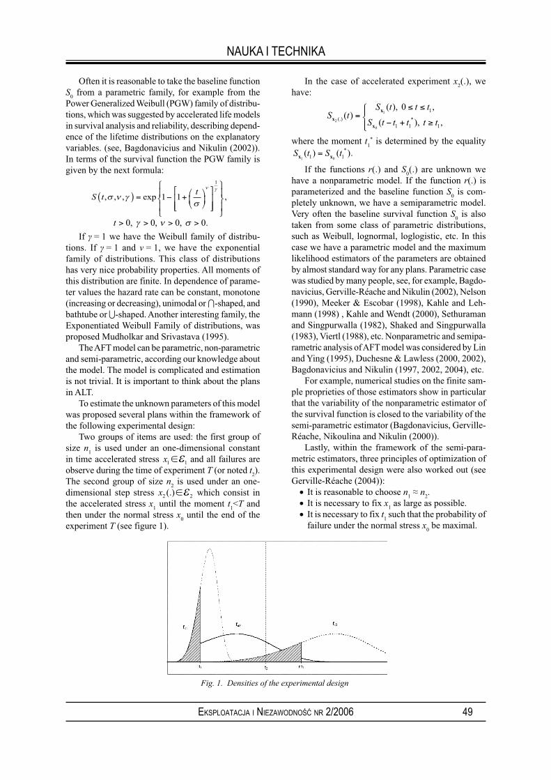
49EKSPLOATACJA I NIEZAWODNOŚĆ NR 2/2006
NAUKA I TECHNIKA
Often it is reasonable to take the baseline function S
0 from a parametric family, for example from the
Power Generalized Weibull (PGW) family of distribu-tions, which was suggested by accelerated life models in survival analysis and reliability, describing depend-ence of the lifetime distributions on the explanatory variables. (see, Bagdonavicius and Nikulin (2002)). In terms of the survival function the PGW family is given by the next formula:
S t
t, , , exp ,σ ν γ
σ
ν γ
( ) = − + ⎛
⎝⎜
⎞
⎠⎟
⎡
⎣⎢⎢
⎤
⎦⎥⎥
⎧
⎨⎪
⎩⎪
⎫
⎬⎪
⎭⎪
1 1
1
t > > > >0 0 0 0, , , .γ ν σ
If γ = 1 we have the Weibull family of distribu-tions. If γ = 1 and v = 1, we have the exponential family of distributions. This class of distributions has very nice probability properties. All moments of this distribution are finite. In dependence of parame-ter values the hazard rate can be constant, monotone (increasing or decreasing), unimodal or ∩-shaped, and bathtube or ∪-shaped. Another interesting family, the Exponentiated Weibull Family of distributions, was proposed Mudholkar and Srivastava (1995).
The AFT model can be parametric, non-parametric and semi-parametric, according our knowledge about the model. The model is complicated and estimation is not trivial. It is important to think about the plans in ALT.
To estimate the unknown parameters of this model was proposed several plans within the framework of the following experimental design:
Two groups of items are used: the first group of size n
1 is used under an one-dimensional constant
in time accelerated stress x1 1∈ε and all failures are observe during the time of experiment T (or noted t
2).
The second group of size n2 is used under an one-
dimensional step stress x2 2(.)∈ε which consist in the accelerated stress x
1 until the moment t
1<T and
then under the normal stress x0 until the end of the
experiment T (see figure 1).
In the case of accelerated experiment x2(.), we
have:
S t
S t t t
S t t t t tx
x
x2
1
0
0 1
1 1 1(.) *( )
( ), ,
( ), ,=
≤ ≤
− + ≥
⎧⎨⎪
⎩⎪
where the moment t1
* is determined by the equality S t S t
x x1 01 1( ) ( )*= .
If the functions r(.) and S0(.) are unknown we
have a nonparametric model. If the function r(.) is parameterized and the baseline function S
0 is com-
pletely unknown, we have a semiparametric model. Very often the baseline survival function S
0 is also
taken from some class of parametric distributions, such as Weibull, lognormal, loglogistic, etc. In this case we have a parametric model and the maximum likelihood estimators of the parameters are obtained by almost standard way for any plans. Parametric case was studied by many people, see, for example, Bagdo-navicius, Gerville-Réache and Nikulin (2002), Nelson (1990), Meeker & Escobar (1998), Kahle and Leh-mann (1998) , Kahle and Wendt (2000), Sethuraman and Singpurwalla (1982), Shaked and Singpurwalla (1983), Viertl (1988), etc. Nonparametric and semipa-rametric analysis of AFT model was considered by Lin and Ying (1995), Duchesne & Lawless (2000, 2002), Bagdonavicius and Nikulin (1997, 2002, 2004), etc.
For example, numerical studies on the finite sam-ple proprieties of those estimators show in particular that the variability of the nonparametric estimator of the survival function is closed to the variability of the semi-parametric estimator (Bagdonavicius, Gerville-Réache, Nikoulina and Nikulin (2000)).
Lastly, within the framework of the semi-para-metric estimators, three principles of optimization of this experimental design were also worked out (see Gerville-Réache (2004)):
• It is reasonable to choose n1 ≈ n
2.
• It is necessary to fix x1 as large as possible.
• It is necessary to fix t1 such that the probability of
failure under the normal stress x0 be maximal.
Fig. 1. Densities of the experimental design

50 EKSPLOATACJA I NIEZAWODNOŚĆ NR 2/2006
NAUKA I TECHNIKA
Model of Sedyakin
In 1966, Sedyakin (1966) formulated his famous physical principle in reliability which states that for two identical populations of units functioning under different stresses x
1 and x
2, two moments t
1 and t
2 are
equivalent if the probabilities of survival until these moments are equal:
P T t S t S t P T tx x x x1 1 2 21 1 2 2≥{ } = = = ≥{ }( ) ( ) ,
x x1 2, ∈εWith the accelerated experiment (1) we have for
all s>0 λ λ
x x1 21 2( ) ( )t s t s+ = +
In ALT is used the model of Sedyakin on ε , based on this idea. Following Bagdonavicius and Nikulin (1995) we give the following definition.
The Sedyakin’s model (SM) holds on a set of stres-ses ε if there exists on ε ×ℜ+ a positive function g such that for all x(.)∈ε
λx x(.) (.)( ) ( ), ( )t g x t t= ( )Λ .
In the case of accelerated experiment x2(.), we
have:
S t
S t t t
S t t t t tx
x
x2
1
0
0 1
1 1 1(.) *( )
( ), ,
( ), ,=
≤ ≤
− + ≥
⎧⎨⎪
⎩⎪
So the AFT model with a stress on ε 2 is the Se-dyakin model.
Changing shape and scale model
Application of the AFT model in the case of the above considered test plan of experiment is considered in Bagdonavicius and Nikulin (2000). Nevertheless, the AFT model is narrow and not always suitable for applications. Natural generalization of the AFT model for constant stresses (see Nelson (1990), Meeker and Escobar (1998)) is obtained by supposing that under different stresses not only scale but shape parameters are different. In this situation is interesting to apply the so-called changing scale and shape (CHSS) model (Bagdonavicius and Nikulin (2002), Bagdonavicius, Nikulin, Zdorova-Cheminade (2004)). The CHSS model holds in a set ε of time-varying stresses if for any x(.)∈ε
S t S r dt
x
xx(.)
( ( ))( ) ( )= { }( )−∫01
0τ τ τν τ ,
where r, v: ε →R+.
In terms of the hazard rate the model can be written in the form :
λ ν
x x
xx(.) (.)
( ( ))( ) ( ) ( )t r t q t t t= { } ( ) −Λ 1
The hazard rate can be monotone (increasing or decreasing) or ∪-shaped. For more details one can see in Bagdonavicius, Nikulin, Zdorova-Cheminade (2004).
References
[1] Bagdonavicius, V., 1978. Testing the hyphothesis of the additive accumulation of damages. Probab. Theory and its Appl., 23, 403-408.
[2] Bagdonavicius, V., Nikulin, M. (1995). Semiparametric models in accelerated life testing. Queen’s Papers in Pure and Applied Mathematics, #98. Queen’s University, Kingston, Canada.
[3] Bagdonavicius, V., Nikulin, M. (1997). Asymptotical Analysis of Semiparametric Models in Survival Analysis
and Accelerated Life Testing. Statistics, 29, #3, 261-284. [4] Bagdonavicius, V., Gerville-Réache, L., Nikoulina, V. and Nikulin, M. (2000). Expériences accélérées: analyse
statistique du modčle standard de vie accélérée. Revue de Statistique Appliquée, XLVIII, #3, 5-38. [5] Bagdonavicius, V., Gerville-Réache, L. and Nikulin, M. (2002). On Parametric Inference for Step-Stress
Models. IEEE Transaction on Reliability, #1, 27-31. [6] Bagdonavicius, V., Nikulin, M. (2002). Accelerated life models. Chapman&Hall/CRC, Boca Raton. [7] Bagdonavicius, V., Nikulin, M., Zdorova-Cheminade, O. (2004). Statistical Planning and Inferencein
Accelerated Life Testing using the CHSS Model. Journal Statistical Planning and Inference, 126, 535-551. [8] Bhattacharyya, G.K., Stoejoeti, Z., 1989. A tampered failure rate model for step-stress accelerated life test,
Comm. in Statist., Theory and Methods, 18, 1627-1643. [9] Ceci, C., Mazliak, L. (2004). Optimal Design in Nonparametric Life Testing. Statistical Inference for Stochastical
Processes, 7, 305-325.[10] Couallier, V. (2004). Comparison of Parameteric and Semiparametric Estimates in a Degradation Model
with Covariates and Traumatic Censoring. In Parametric and Semiparametric Models with Applications to Reliability, Survival Analysis, and Quality of Life, (M.Nikulin, N.Balakrishnan, M.Mesbah, N.Limnios, eds.) Birkhauser, Boston, 81-98.
[11] Duchesne, T. (2000). Methods Common to Reliability and Survival Analysis. In Recent Advances in Reliability Theory, ( N. Limnios and M. Nikulin, eds.) Birkhauser, Boston, 279-290.

51EKSPLOATACJA I NIEZAWODNOŚĆ NR 2/2006
NAUKA I TECHNIKA
[12] Duchesne, T., Rosenthal, J.B. (2003). On the collapsibility of lifetime regression models. Advances in Applied Probability, 35, 755-772.
[13] Duchesne, T., Lawless, J. (2000). Alternative Time Scale and Failure Time Models. Lifetime Data Analysis, 6, 157-179.
[14] Duchesne, T. and Lawless, J. (2002). Semiparametric inference methods for general time scale models. Lifetime Data Analysis, 8, 263-276.
[15] Elasayed, E.A., Liao,H.T. (2004). Reliability Prediction and Testing Plan Based on an Accelerated Degradation
Rate Model. International Journal of Materials & Product Technology, 21, 5, 402-422.[16] Gerville-Réache, L. (2004). An example of optimal design in accelerated experiment. In Parametric and
Semiparametric Models with Applications to Reliability, Survival Analysis, and Quality of Life, (M.Nikulin, N.Balakrishnan, M.Mesbah, N.Limnios, eds.) Birkhauser, Boston,, 121-131.
[17] Greenwood, P.E., Nikulin,M. (1996). A Guide to Chi-squared Testing, John Wiley and Sons: New York.[18] Kahle, W., Lehmann, A. (1998). Parameter Estimation in Damage Processes: dependent observation of
damage increments and first passage time. In Advances in Stochastic Models for Reliability, Quality and Safety. (W.Kahle, E. Collant, J. Franz and U. Jensen, eds.) Birkhauser: Boston, 139-152.
[19] Kahle, W., Wendt, H. (2000). Statistical analysis of damage processes. In Recent Advances in Reliability Theory, ( N. Limnios and M. Nikulin, eds.) Birkhauser, Boston, 199-212.
[20] Lawless, J.F. (2000). Dynamic Analysis of Failures in Repairable Systems and Software. In Recent Advances in Reliability Theory. (N. Limnios and M. Nikulin, eds). Birkhauser, Boston, 341-354.
[21] Lawless, J.F. (2003). Statistical Models and Methods for Lifetime Data. Second Edition, John Wiley: New York.
[22] Lehmann, A. (2004). On Degradation-Failure Model for Repairable Items. In Parametric and Semiparametric Models with Applications to Reliability, Survival Analysis, and Quality of Life, (M.Nikulin, N.Balakrishnan, M.Mesbah, N.Limnios, eds.) Birkhauser, Boston, 65-79.
[23] Lin, D.Y. and Ying, Z. (1995). Semiparametric inference for accelerated life model with time dependent
covariates. Journal of Statist. Planning and Inference, 44, 47-63.[24] LuValle, M. (2000). A Theoretical Framework for Accelerated Testing. In Recent Advances in Reliability
Theory. (N. Limnios and M. Nikulin, eds). Birkhauser, Boston, 419-434.[25] Meeker, W., Escobar, L. (1998). Statistical Methods for Reliability Data. Wiley, New York.[26] Mudholkar, G., Srivastava, D. (1995). The exponentiated Weibull Family: A Reanalysis of the Bus-Motor-
Failure Data. Technometrics, 37, \#14, 436-445.[27] Nelson, W. (1990). Accelerated Testing: Statistical Models, Test Plans, and Data Analysis. Wiley, New York.[28] Nikulin M., Balakrishnan N., Mesbah M., Limnios N. (eds) (2004). Parametric and Semiparametric Models
with Applications to Reliability, Survival Analysis, and Quality of Life, Birkhauser, Boston.[29] Nikulin, M., Gerville-Réache, L., Orazio, S.. About one parametric degradation model used in reliability, survival
analysis and quality of life. In: Advances in Statistical Methods for Health Sciences, Eds : Balakhrishnan, Auget, Mesbah, Molenberghs. Springer (to appear) 11p.
[30] Sedyakin, N.M. (1966). On one physical principle in reliability theory. (in Russian). Techn. Cybernetics, 3, 80-87.
[31] Sethuraman, J. and Singpurwalla, N.D. (1982). Testing of hypotheses for distributions in accelerated life tests. JASA, 77, 204-208.
[32] Shaked, M. and Singpurwalla, N.D. (1983). Inference for step-stress accelerated life tests. J. Statist. Plann. Inference, 7, 295-306.
[33] Singpurwalla, N. (1995). Survival in Dynamic Environments. Statistical Sciences, 1, 86-103.[34] Viertl, R. (1988). Statistical Methods in Accelerated Life Testing. Vandenhoeck and Ruprecht. Goettingen.[35] Zhao, W., Elsayed, E.A. (2003). An Accelerated Life Testing Under Competing Failure Modes. Paper 2003-
128, Rutgers University.
Ph.D. Prof. Léo GERVILLE-RÉACHEPh.D. Prof. Mikhail NIKULINStatistique Mathématique et ses ApplicationsVictor Segalen University Bordeaux 2, Bordeaux, 33076, Francee-mail: [email protected] / [email protected]

52 EKSPLOATACJA I NIEZAWODNOŚĆ NR 2/2006
Andrzej NIEWCZASGrzegorz KOSZAŁKAPawel DROŹDZIEL
STOCHASTIC MODEL OF TRUCK ENGINE WEAR WITH REGARD TO DI-
SCONTINUITY OF OPERATION
The influence of operational factors on the wear process of the truck engine parts was analysed.
Discontinuity of engine operation was found to be a crucial factor. Contribution of start-ups,
following breaks in operation in total wear of the engine is significant and in case of investigated
engine amounts 40%. As wear of engine parts accompanying a single start-up strongly depends
on the temperature, cold start-ups (usually first in the morning) are of particular importance.
Taking above into consideration the authors suggest modelling the course of wear as a stochastic
process with the following constituents:
– transmission process with linear realization representing average value of wear,
– stationary process with periodical realization representing deviations of wear intensity in
particular seasons accompanying cold start-ups,
– stationary process of statistic fluctuations with random time realizations, representing
instantaneous deviations of wear in relation to average values.
Mathematical model was illustrated with some empirical results.
Keywords: diesel engine, wear, cylinder liner, durability prediction
1. Introduction
Stochastic models of mechanical wear of engine cylinders are frequently used for accelerated investi-gations of engine durability. Such models most often describe growth-rate of cylinder diameter as a function of vehicle operation time.
Analysing process of friction, which is the cause of cylinder wear, it can be assumed that this wear is a sum of three separate components. The first component is wear occurring during quasi-steady, continuous engine operation. In such conditions wear intensity of cylin-der liner is relatively small. The second component is so called start-up wear. It takes place only during putting engine in motion. The third component are random processes of surface degradation produced by instantaneous random inputs. Increments of wear caused by this component are rather small.
2. Mathematical model
The mathematical model was worked out on the basis of already described foundations (Niewczas 1989, Niewczas 1993):
Z Z Vt A t tt z r j= + + +( ) + ( )0 sin ω φ ΣΔΨ (1)
where: Zt – non-stationary stochastic wear process,
Z0, V – variables independent of time, where Z
0 is initial
wear and V is stabilized wear intensity, Azsin(ωt+φ)
– one-dimensional stationary process with periodic re-
alization, where both amplitude Az and pulsation ω are
constant, but the initial phase φ is arandom variable with uniform distribution, ΣΔΨ
r(t
j) – one-dimensio-
nal, normal stationary process with expected value of zero and random variable realization, t – time, t ∈ [t
p,
tm], where t
p ≥ 0 is the initial time and t
m denotes the
moment of exceeding the limit wear.The model consists of three units. The expression
Z0 + Vt constitutes the first unit, and is the evolutionary
constituent of the wear – this unit is also named as the transmission process. Transmission process describes average wear change observed in long period of time, and is a sum of quasi-steady and start-up wear.
The second unit represented by the expression A
zsin(ωt+φ) = Ψ
ωt constitutes periodical component
of wear changes, which describes cyclic deviations of wear from the value determined by the transmission process. In described model it is assumed that this deviations mostly results from different temperatures of cold start-ups (usually only the first start-up in the morning, at most two start-ups a day) in particular seasons.
The third unit, namely expression ΣΔΨr(t
j) = Ψ
rt
constitutes the random component of the wear changes – also named as the random fluctuation process. Fig. 1 presents the model described above.
The model gives new explanations of the reasons responsible for the origin of failures of tribological systems in IC engines. Exceeding the limit wear by the
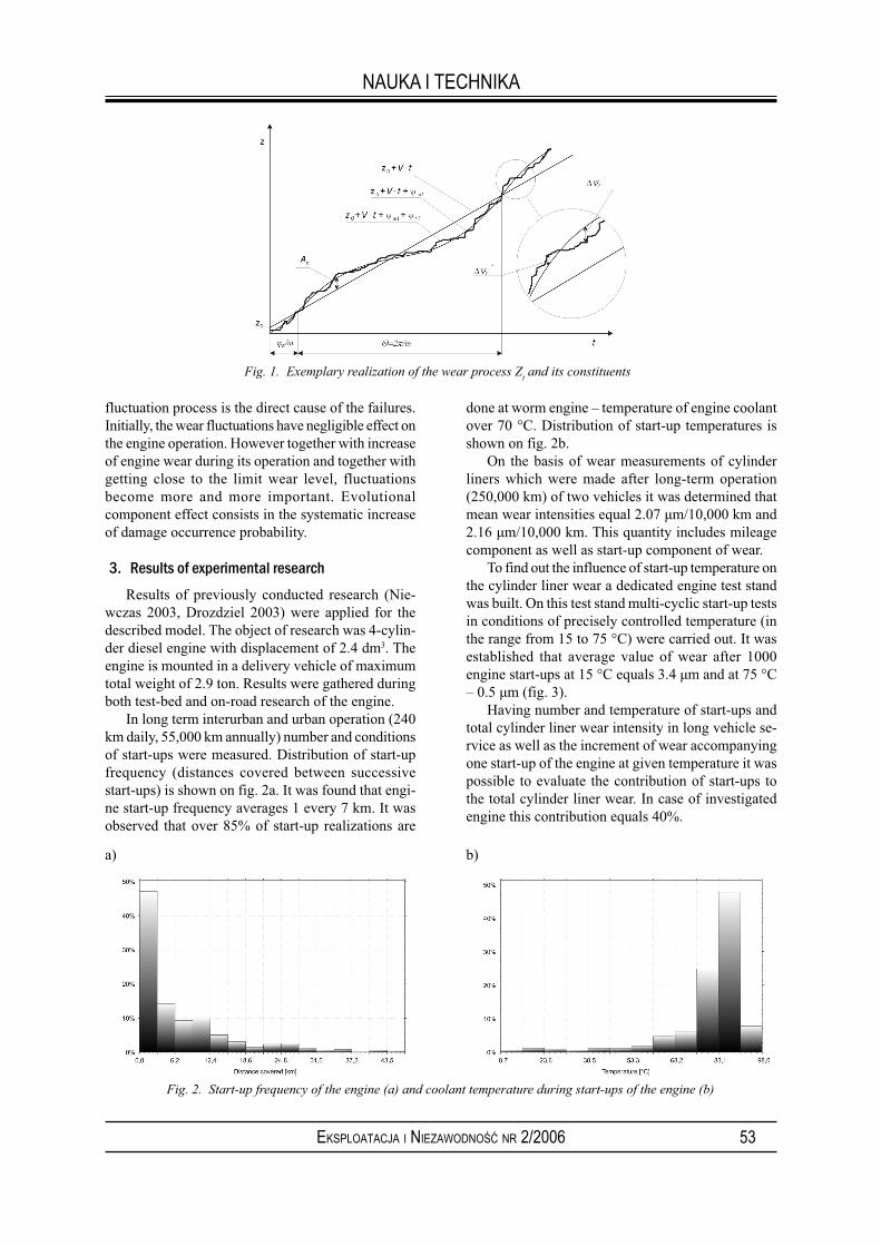
53EKSPLOATACJA I NIEZAWODNOŚĆ NR 2/2006
NAUKA I TECHNIKA
fluctuation process is the direct cause of the failures. Initially, the wear fluctuations have negligible effect on the engine operation. However together with increase of engine wear during its operation and together with getting close to the limit wear level, fluctuations become more and more important. Evolutional component effect consists in the systematic increase of damage occurrence probability.
3. Results of experimental research
Results of previously conducted research (Nie-wczas 2003, Drozdziel 2003) were applied for the described model. The object of research was 4-cylin-der diesel engine with displacement of 2.4 dm3. The engine is mounted in a delivery vehicle of maximum total weight of 2.9 ton. Results were gathered during both test-bed and on-road research of the engine.
In long term interurban and urban operation (240 km daily, 55,000 km annually) number and conditions of start-ups were measured. Distribution of start-up frequency (distances covered between successive start-ups) is shown on fig. 2a. It was found that engi-ne start-up frequency averages 1 every 7 km. It was observed that over 85% of start-up realizations are
done at worm engine – temperature of engine coolant over 70 °C. Distribution of start-up temperatures is shown on fig. 2b.
On the basis of wear measurements of cylinder liners which were made after long-term operation (250,000 km) of two vehicles it was determined that mean wear intensities equal 2.07 μm/10,000 km and 2.16 μm/10,000 km. This quantity includes mileage component as well as start-up component of wear.
To find out the influence of start-up temperature on the cylinder liner wear a dedicated engine test stand was built. On this test stand multi-cyclic start-up tests in conditions of precisely controlled temperature (in the range from 15 to 75 °C) were carried out. It was established that average value of wear after 1000 engine start-ups at 15 °C equals 3.4 μm and at 75 °C – 0.5 μm (fig. 3).
Having number and temperature of start-ups and total cylinder liner wear intensity in long vehicle se-rvice as well as the increment of wear accompanying one start-up of the engine at given temperature it was possible to evaluate the contribution of start-ups to the total cylinder liner wear. In case of investigated engine this contribution equals 40%.
Fig. 1. Exemplary realization of the wear process Zt and its constituents
Fig. 2. Start-up frequency of the engine (a) and coolant temperature during start-ups of the engine (b)
a) b)
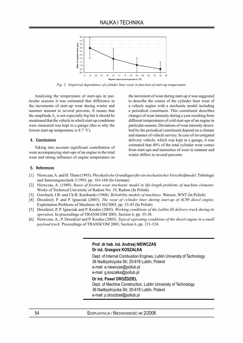
54 EKSPLOATACJA I NIEZAWODNOŚĆ NR 2/2006
NAUKA I TECHNIKA
Analysing the temperature of start-ups in par-ticular seasons it was estimated that difference in the increments of start-up wear during winter and summer amount to several percents. It means that the amplitude A
z is not especially big but it should be
mentioned that the vehicle in which start-up conditions were measured was kept in a garage (this is why the lowest start-up temperature is 8.7 °C).
4. Conclusions
Taking into account significant contribution of wear accompanying start-ups of an engine to the total wear and strong influence of engine temperature on
the increment of wear during start-up it was suggested to describe the course of the cylinder liner wear of a vehicle engine with a stochastic model including a periodical constituent. This constituent describes changes of wear intensity during a year resulting from different temperatures of cold start-ups of an engine in particular seasons. Deviations of wear intensity descri-bed by the periodical constituent depend on a climate and manner of vehicle service. In case of investigated delivery vehicle, which was kept in a garage, it was estimated that 40% of the total cylinder wear comes from start-ups and intensities of wear in summer and winter differs in several percents.
Fig. 3. Empirical dependence of cylinder liner wear in function of start-up temperature
5. References
[1] Niewczas, A. and H. Thum (1993). Physikalische Grundlagen für ein stochastisches Verschleiβmodel. Tribologie und Smierungstechnik 3/1993, pp. 163-168 (In German).
[2] Niewczas, A. (1989). Bases of friction wear stochastic model in life-length problems of machine elements. Works of Technical University of Radom No. 19, Radom (In Polish).
[3] Gercbach, I.B. and Ch.B. Kordonski (1968). Reliability models of machines. Warsaw, WNT (In Polish).[4] Drozdziel, P. and P. Ignaciuk (2003). The wear of cylinder liner during start-up of 4C90 diesel engine.
Exploitation Problems of Machines 4(136)/2003, pp. 33-43 (In Polish).[5] Drozdziel, P, P. Ignaciuk and P. Kordos (2003). Working conditions of the Lublin III delivery truck during its
operation. In proceedings of TRANSCOM 2003, Section 6, pp. 35-38.[6] Niewczas, A., P. Drozdziel and P. Kordos (2003). Typical operating conditions of the diesel engine in a small
payload truck. Proceedings of TRANSCOM 2003, Section 6, pp. 121-124.
Prof. dr hab. inż. Andrzej NIEWCZASDr inż. Grzegorz KOSZAŁKA
Dept. of Internal Combustion Engines, Lublin University of Technology36 Nadbystrzycka Str, 20-618 Lublin, Polande-mail: [email protected]: [email protected]
Dr inż. Pawel DROŹDZIELDept. of Machine Construction, Lublin University of Technology36 Nadbystrzycka Str, 20-618 Lublin, Polande-mail: [email protected]