Embed Size (px)
Citation preview

1
1Slide© 2005 Thomson/South-Western
Slides Prepared byJOHN S. LOUCKS
St. Edward’s University
2Slide© 2005 Thomson/South-Western
Chapter 6Continuous Probability Distributions
� Uniform Probability Distribution� Normal Probability Distribution� Exponential Probability Distribution
f (x)
x
Uniform
x
f (x) Normal
x
f (x) Exponential
3Slide© 2005 Thomson/South-Western
Continuous Probability Distributions
� A continuous random variable can assume any value in an interval on the real line or in a collection of intervals.
� It is not possible to talk about the probability of the random variable assuming a particular value.
� Instead, we talk about the probability of the random variable assuming a value within a given interval.

2
4Slide© 2005 Thomson/South-Western
Continuous Probability Distributions
� The probability of the random variable assuming a value within some given interval from x1 to x2 is defined to be the area under the graph of the probability density function between x1 and x2.
f (x)
x
Uniform
x1 x2
x
f (x) Normal
x1 x2
x1 x2
Exponential
x
f (x)
x1 x2
5Slide© 2005 Thomson/South-Western
Uniform Probability Distribution
where: a = smallest value the variable can assumeb = largest value the variable can assume
f (x) = 1/(b – a) for a < x < b= 0 elsewhere
� A random variable is uniformly distributedwhenever the probability is proportional to the interval’s length.
� The uniform probability density function is:
6Slide© 2005 Thomson/South-Western
Var(x) = (b - a)2/12
E(x) = (a + b)/2
Uniform Probability Distribution
� Expected Value of x
� Variance of x

3
7Slide© 2005 Thomson/South-Western
Uniform Probability Distribution
� Example: Slater's BuffetSlater customers are charged
for the amount of salad they take. Sampling suggests that theamount of salad taken is uniformly distributedbetween 5 ounces and 15 ounces.
8Slide© 2005 Thomson/South-Western
� Uniform Probability Density Function
f(x) = 1/10 for 5 < x < 15= 0 elsewhere
where:x = salad plate filling weight
Uniform Probability Distribution
9Slide© 2005 Thomson/South-Western
� Expected Value of x
� Variance of x
E(x) = (a + b)/2= (5 + 15)/2= 10
Var(x) = (b - a)2/12= (15 – 5)2/12= 8.33
Uniform Probability Distribution

4
10Slide© 2005 Thomson/South-Western
� Uniform Probability Distributionfor Salad Plate Filling Weight
f(x)
x5 10 15
1/10
Salad Weight (oz.)
Uniform Probability Distribution
11Slide© 2005 Thomson/South-Western
f(x)
x5 10 15
1/10
Salad Weight (oz.)
P(12 < x < 15) = 1/10(3) = .3
What is the probability that a customerwill take between 12 and 15 ounces of salad?
12
Uniform Probability Distribution
12Slide© 2005 Thomson/South-Western
Normal Probability Distribution
� The normal probability distribution is the most important distribution for describing a continuous random variable.
� It is widely used in statistical inference.

5
13Slide© 2005 Thomson/South-Western
Heightsof people
Normal Probability Distribution
� It has been used in a wide variety of applications:
Scientificmeasurements
14Slide© 2005 Thomson/South-Western
Amountsof rainfall
Normal Probability Distribution
� It has been used in a wide variety of applications:
Testscores
15Slide© 2005 Thomson/South-Western
Normal Probability Distribution
� Normal Probability Density Function
2 2( ) /21( )2
xf x e µ σ
σ π− −=
2 2( ) /21( )2
xf x e µ σ
σ π− −=
µ = meanσ = standard deviationπ = 3.14159e = 2.71828
where:

6
16Slide© 2005 Thomson/South-Western
The distribution is symmetric; its skewnessmeasure is zero.
Normal Probability Distribution
� Characteristics
x
17Slide© 2005 Thomson/South-Western
The entire family of normal probabilitydistributions is defined by its mean µ and itsstandard deviation σ .
Normal Probability Distribution
� Characteristics
Standard Deviation σ
Mean µx
18Slide© 2005 Thomson/South-Western
The highest point on the normal curve is at themean, which is also the median and mode.
Normal Probability Distribution
� Characteristics
x
7
19Slide© 2005 Thomson/South-Western
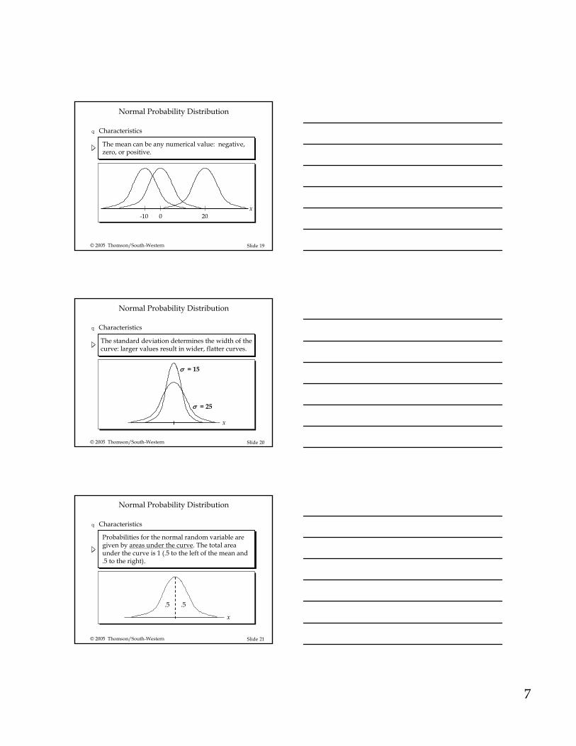
Normal Probability Distribution
� Characteristics
-10 0 20
The mean can be any numerical value: negative,zero, or positive.
x
20Slide© 2005 Thomson/South-Western
Normal Probability Distribution
� Characteristics
σ = 15
σ = 25
The standard deviation determines the width of thecurve: larger values result in wider, flatter curves.
x
21Slide© 2005 Thomson/South-Western
Probabilities for the normal random variable aregiven by areas under the curve. The total areaunder the curve is 1 (.5 to the left of the mean and.5 to the right).
Normal Probability Distribution
� Characteristics
.5 .5
x

8
22Slide© 2005 Thomson/South-Western
Normal Probability Distribution
� Characteristics
of values of a normal random variableare within of its mean.68.26%
+/- 1 standard deviation
of values of a normal random variableare within of its mean.95.44%
+/- 2 standard deviations
of values of a normal random variableare within of its mean.99.72%
+/- 3 standard deviations
23Slide© 2005 Thomson/South-Western
Normal Probability Distribution
� Characteristics
xµ – 3σ µ – 1σ
µ – 2σµ + 1σ
µ + 2σµ + 3σµ
68.26%95.44%99.72%
24Slide© 2005 Thomson/South-Western
Standard Normal Probability Distribution
A random variable having a normal distributionwith a mean of 0 and a standard deviation of 1 issaid to have a standard normal probabilitydistribution.

9
25Slide© 2005 Thomson/South-Western
σ = 1
0z
The letter z is used to designate the standardnormal random variable.
Standard Normal Probability Distribution
26Slide© 2005 Thomson/South-Western
� Converting to the Standard Normal Distribution
Standard Normal Probability Distribution
z x=
− µσ
z x=
− µσ
We can think of z as a measure of the number ofstandard deviations x is from µ.
27Slide© 2005 Thomson/South-Western
Standard Normal Probability Distribution
� Standard Normal Density Function
π−=
2 /21( )2
zf x eπ
−=2 /21( )
2zf x e
z = (x – µ)/σπ = 3.14159e = 2.71828
where:

10
28Slide© 2005 Thomson/South-Western
Standard Normal Probability Distribution
� Example: Pep ZonePep Zone sells auto parts and supplies including
a popular multi-grade motor oil. When thestock of this oil drops to 20 gallons, areplenishment order is placed.
PepZone5w-20
Motor Oil
29Slide© 2005 Thomson/South-Western
The store manager is concerned that sales are beinglost due to stockouts while waiting for an order.It has been determined that demand duringreplenishment lead-time is normallydistributed with a mean of 15 gallons anda standard deviation of 6 gallons.
The manager would like to know theprobability of a stockout, P(x > 20).
Standard Normal Probability Distribution
PepZone5w-20
Motor Oil
� Example: Pep Zone
30Slide© 2005 Thomson/South-Western
z = (x - µ)/σ= (20 - 15)/6= .83
� Solving for the Stockout Probability
Step 1: Convert x to the standard normal distribution.
PepZone
5w-20Motor Oil
Step 2: Find the area under the standard normalcurve to the left of z = .83.
see next slide
Standard Normal Probability Distribution

11
31Slide© 2005 Thomson/South-Western
� Cumulative Probability Table for the Standard Normal Distribution
z .00 .01 .02 .03 .04 .05 .06 .07 .08 .09. . . . . . . . . . ..5 .6915 .6950 .6985 .7019 .7054 .7088 .7123 .7157 .7190 .7224.6 .7257 .7291 .7324 .7357 .7389 .7422 .7454 .7486 .7517 .7549.7 .7580 .7611 .7642 .7673 .7704 .7734 .7764 .7794 .7823 .7852.8 .7881 .7910 .7939 .7967 .7995 .8023 .8051 .8078 .8106 .8133.9 .8159 .8186 .8212 .8238 .8264 .8289 .8315 .8340 .8365 .8389. . . . . . . . . . .
PepZone
5w-20Motor Oil
P(z < .83)
Standard Normal Probability Distribution
32Slide© 2005 Thomson/South-Western
P(z > .83) = 1 – P(z < .83) = 1- .7967
= .2033
� Solving for the Stockout Probability
Step 3: Compute the area under the standard normalcurve to the right of z = .83.
PepZone
5w-20Motor Oil
Probabilityof a stockout P(x > 20)
Standard Normal Probability Distribution
33Slide© 2005 Thomson/South-Western
� Solving for the Stockout Probability
0 .83
Area = .7967Area = 1 - .7967
= .2033
z
PepZone
5w-20Motor Oil
Standard Normal Probability Distribution

12
34Slide© 2005 Thomson/South-Western
� Standard Normal Probability DistributionIf the manager of Pep Zone wants the probability
of a stockout to be no more than .05, what should the reorder point be?
PepZone
5w-20Motor Oil
Standard Normal Probability Distribution
35Slide© 2005 Thomson/South-Western
� Solving for the Reorder Point
PepZone
5w-20Motor Oil
0
Area = .9500
Area = .0500
zz.05
Standard Normal Probability Distribution
36Slide© 2005 Thomson/South-Western
� Solving for the Reorder Point
PepZone
5w-20Motor Oil
Step 1: Find the z-value that cuts off an area of .05in the right tail of the standard normaldistribution.
z .00 .01 .02 .03 .04 .05 .06 .07 .08 .09. . . . . . . . . . .
1.5 .9332 .9345 .9357 .9370 .9382 .9394 .9406 .9418 .9429 .94411.6 .9452 .9463 .9474 .9484 .9495 .9505 .9515 .9525 .9535 .95451.7 .9554 .9564 .9573 .9582 .9591 .9599 .9608 .9616 .9625 .96331.8 .9641 .9649 .9656 .9664 .9671 .9678 .9686 .9693 .9699 .97061.9 .9713 .9719 .9726 .9732 .9738 .9744 .9750 .9756 .9761 .9767 . . . . . . . . . . .
We look up the complement of the tail area (1 - .05 = .95)
Standard Normal Probability Distribution

13
37Slide© 2005 Thomson/South-Western
� Solving for the Reorder Point
PepZone
5w-20Motor Oil
Step 2: Convert z.05 to the corresponding value of x.
x = µ + z.05σ = 15 + 1.645(6)
= 24.87 or 25
A reorder point of 25 gallons will place the probabilityof a stockout during leadtime at (slightly less than) .05.
Standard Normal Probability Distribution
38Slide© 2005 Thomson/South-Western
� Solving for the Reorder Point
PepZone
5w-20Motor Oil
By raising the reorder point from 20 gallons to 25 gallons on hand, the probability of a stockoutdecreases from about .20 to .05.
This is a significant decrease in the chance that PepZone will be out of stock and unable to meet acustomer’s desire to make a purchase.
Standard Normal Probability Distribution
39Slide© 2005 Thomson/South-Western
Normal Approximation of Binomial Probabilities
When the number of trials, n, becomes large,evaluating the binomial probability function byhand or with a calculator is difficult
The normal probability distribution provides aneasy-to-use approximation of binomial probabilitieswhere n > 20, np > 5, and n(1 - p) > 5.

14
40Slide© 2005 Thomson/South-Western
Normal Approximation of Binomial Probabilities
� Set µ = np
σ = −(1 )np pσ = −(1 )np p
� Add and subtract 0.5 (a continuity correction factor)because a continuous distribution is being used toapproximate a discrete distribution. For example, P(x = 10) is approximated by P(9.5 < x < 10.5).
41Slide© 2005 Thomson/South-Western
Exponential Probability Distribution
� The exponential probability distribution is useful in describing the time it takes to complete a task.
� The exponential random variables can be used to describe:
Time betweenvehicle arrivalsat a toll booth
Time requiredto complete
a questionnaire
Distance betweenmajor defectsin a highway
SLOW
42Slide© 2005 Thomson/South-Western
� Density Function
Exponential Probability Distribution
where: µ = meane = 2.71828
f x e x( ) /= −1µ
µf x e x( ) /= −1µ
µ for x > 0, µ > 0

15
43Slide© 2005 Thomson/South-Western
� Cumulative Probabilities
Exponential Probability Distribution
P x x e x( ) /≤ = − −0 1 o µP x x e x( ) /≤ = − −0 1 o µ
where:x0 = some specific value of x
44Slide© 2005 Thomson/South-Western
Exponential Probability Distribution
� Example: Al’s Full-Service PumpThe time between arrivals of cars
at Al’s full-service gas pump followsan exponential probability distributionwith a mean time between arrivals of 3 minutes. Al would like to know theprobability that the time between two successivearrivals will be 2 minutes or less.
45Slide© 2005 Thomson/South-Western
x
f(x)
.1
.3
.4
.2
1 2 3 4 5 6 7 8 9 10Time Between Successive Arrivals (mins.)
Exponential Probability Distribution
P(x < 2) = 1 - 2.71828-2/3 = 1 - .5134 = .4866

16
46Slide© 2005 Thomson/South-Western
Exponential Probability Distribution
A property of the exponential distribution is thatthe mean, µ, and standard deviation, σ, are equal.
Thus, the standard deviation, σ, and variance, σ 2, forthe time between arrivals at Al’s full-service pump are:
σ = µ = 3 minutes
σ 2 = (3)2 = 9
47Slide© 2005 Thomson/South-Western
Exponential Probability Distribution
The exponential distribution is skewed to the right.
The skewness measure for the exponential distributionis 2.
48Slide© 2005 Thomson/South-Western
Relationship between the Poissonand Exponential Distributions
The Poisson distributionprovides an appropriate description
of the number of occurrencesper interval
The exponential distributionprovides an appropriate description
of the length of the intervalbetween occurrences

17
49Slide© 2005 Thomson/South-Western
End of Chapter 6